UPDATE: See Generative Models in Tensorflow 2 for a Tensorflow 2.X version of VAEGAN.

Tensorflow Multi-GPU VAE-GAN implementation

• This is an implementation of the VAE-GAN based on the implementation described in <a href="http://arxiv.org/abs/1512.09300">Autoencoding beyond pixels using a learned similarity metric</a>
• I implement a few useful things like
  • Visualizing Movement Through Z-Space
  • Latent Space Algebra
  • Spike Triggered Average Style Receptive Fields

How does a VAE-GAN work?

• We have three networks, an <font color="#38761d"><strong>Encoder</strong></font>, a <font color="#1155cc"><strong>Generator</strong></font>, and a <font color="#ff0000"><strong>Discriminator</strong></font>.
  • The <font color="#38761d"><strong>Encoder</strong></font> learns to map input x onto z space (latent space)
  • The <font color="#1155cc"><strong>Generator</strong></font> learns to generate x from z space
  • The <font color="#ff0000"><strong>Discriminator</strong></font> learns to discriminate whether the image being put in is real, or generated

Diagram of basic network input and output

l_x_tilde and l_x here become layers of high level features that the discriminator learns.

• we train the network to minimize the difference between the high level features of x and x_tilde
• This is basically an autoencoder that works on high level features rather than pixels
• Adding this autoencoder to a GAN helps to stabilize the GAN

Training

Train <font color="#38761d"><strong>Encoder</strong></font> on minimization of:

• kullback_leibler_loss(z_x, gaussian)
• mean_squared_error(l_x_tilde_, l_x)

Train <font color="#1155cc"><strong>Generator</strong></font> on minimization of:

• kullback_leibler_loss(z_x, gaussian)
• mean_squared_error(l_x_tilde_, l_x)
• -1*log(d_x_p)

Train <font color="#ff0000"><strong>Discriminator</strong></font> on minimization of:

• -1*log(d_x) + log(1 - d_x_p)

# Import all of our packages

import os
import numpy as np
import prettytensor as pt
import tensorflow as tf
from tensorflow.examples.tutorials.mnist import input_data
import matplotlib.pyplot as plt
from deconv import deconv2d
import IPython.display
import math
import tqdm # making loops prettier
import h5py # for reading our dataset
import ipywidgets as widgets
from ipywidgets import interact, interactive, fixed

%matplotlib inline  

Parameters

dim1 = 64 # first dimension of input data
dim2 = 64 # second dimension of input data
dim3 = 3 # third dimension of input data (colors)
batch_size = 32 # size of batches to use (per GPU)
hidden_size = 2048 # size of hidden (z) layer to use
num_examples = 60000 # how many examples are in your training set
num_epochs = 10000 # number of epochs to run
### we can train our different networks  with different learning rates if we want to
e_learning_rate = 1e-3
g_learning_rate = 1e-3
d_learning_rate = 1e-3

Which GPUs are we using?

• Set gpus to a list of the GPUs you're using. The network will then split up the work between those gpus

gpus = [2] # Here I set CUDA to only see one GPU
os.environ["CUDA_VISIBLE_DEVICES"]=','.join([str(i) for i in gpus])
num_gpus = len(gpus) # number of GPUs to use

Reading the dataset from HDF5 format

• open `makedataset.ipynb' for instructions on how to build the dataset

with h5py.File(''.join(['datasets/faces_dataset_new.h5']), 'r') as hf:
    faces = hf['images'].value
    headers = hf['headers'].value
    labels = hf['label_input'].value

# Normalize the dataset between 0 and 1
faces = (faces/255.)

# Just taking a look and making sure everything works
plt.imshow(np.reshape(faces[1], (64,64,3)), interpolation='nearest')

<matplotlib.image.AxesImage at 0x7fe6bc24ce50>

# grab the faces back out after we've flattened them
def create_image(im):
    return np.reshape(im,(dim1,dim2,dim3))

# Lets just take a look at our channels
cm = plt.cm.hot
test_face = faces[0].reshape(dim1,dim2,dim3)
fig, ax = plt.subplots(nrows=1,ncols=4, figsize=(20,8))
ax[0].imshow(create_image(test_face), interpolation='nearest')
ax[1].imshow(create_image(test_face)[:,:,0], interpolation='nearest', cmap=cm)
ax[2].imshow(create_image(test_face)[:,:,1], interpolation='nearest', cmap=cm)
ax[3].imshow(create_image(test_face)[:,:,2], interpolation='nearest', cmap=cm)

<matplotlib.image.AxesImage at 0x7fe6ad0a9150>

A data iterator for batching (drawn up by Luke Metz)

• https://indico.io/blog/tensorflow-data-inputs-part1-placeholders-protobufs-queues/

def data_iterator():
    """ A simple data iterator """
    batch_idx = 0
    while True:
        idxs = np.arange(0, len(faces))
        np.random.shuffle(idxs)
        for batch_idx in range(0, len(faces), batch_size):
            cur_idxs = idxs[batch_idx:batch_idx+batch_size]
            images_batch = faces[cur_idxs]
            #images_batch = images_batch.astype("float32")
            labels_batch = labels[cur_idxs]
            yield images_batch, labels_batch

            
iter_ = data_iterator()

iter_ = data_iterator()

#face_batch, label_batch

Bald people

fig, ax = plt.subplots(nrows=1,ncols=4, figsize=(20,8))
ax[0].imshow(create_image(faces[labels[:,4] == 1][0]), interpolation='nearest')
ax[1].imshow(create_image(faces[labels[:,4] == 1][1]), interpolation='nearest')
ax[2].imshow(create_image(faces[labels[:,4] == 1][2]), interpolation='nearest')
ax[3].imshow(create_image(faces[labels[:,4] == 1][3]), interpolation='nearest')

<matplotlib.image.AxesImage at 0x7fe6aabff650>

Draw out the architecture of our network

• Each of these functions represent the <font color="#38761d"><strong>Encoder</strong></font>, <font color="#1155cc"><strong>Generator</strong></font>, and <font color="#ff0000"><strong>Discriminator</strong></font> described above.
• It would be interesting to try and implement the inception architecture to do the same thing, next time around: <br /><br />
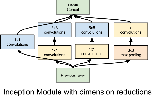
• They describe how to implement inception, in prettytensor, here: https://github.com/google/prettytensor

def encoder(X):
    '''Create encoder network.
    Args:
        x: a batch of flattened images [batch_size, 28*28]
    Returns:
        A tensor that expresses the encoder network
            # The transformation is parametrized and can be learned.
            # returns network output, mean, setd
    '''
    lay_end = (pt.wrap(X).
            reshape([batch_size, dim1, dim2, dim3]). 
            conv2d(5, 64, stride=2). 
            conv2d(5, 128, stride=2). 
            conv2d(5, 256, stride=2). 
            flatten())
    z_mean = lay_end.fully_connected(hidden_size, activation_fn=None)
    z_log_sigma_sq = lay_end.fully_connected(hidden_size, activation_fn=None)
    return z_mean, z_log_sigma_sq


def generator(Z):
    '''Create generator network.
        If input tensor is provided then decodes it, otherwise samples from 
        a sampled vector.
    Args:
        x: a batch of vectors to decode
    Returns:
        A tensor that expresses the generator network
    '''
    return (pt.wrap(Z).
            fully_connected(8*8*256).reshape([batch_size, 8, 8, 256]). #(128, 4 4, 256)
            deconv2d(5, 256, stride=2).
            deconv2d(5, 128, stride=2).
            deconv2d(5, 32, stride=2).
            deconv2d(1, dim3, stride=1, activation_fn=tf.sigmoid).
            flatten()
           )



def discriminator(D_I):
    ''' A encodes
    Create a network that discriminates between images from a dataset and
    generated ones.
    Args:
        input: a batch of real images [batch, height, width, channels]
    Returns:
        A tensor that represents the network
    ''' 
    descrim_conv =  (pt.wrap(D_I). # This is what we're descriminating
            reshape([batch_size, dim1, dim2, dim3]).
            conv2d(5, 32, stride=1).
            conv2d(5, 128, stride=2).
            conv2d(5, 256, stride=2).
            conv2d(5, 256, stride=2).
            flatten()
            )
    lth_layer= descrim_conv.fully_connected(1024, activation_fn=tf.nn.elu)# this is the lth layer       
    D =lth_layer.fully_connected(1, activation_fn=tf.nn.sigmoid) # this is the actual discrimination
    return D, lth_layer

Defining the forward pass through the network

• This function is based upon the inference function from tensorflows cifar tutorials
  • https://github.com/tensorflow/tensorflow/blob/r0.10/tensorflow/models/image/cifar10/cifar10.py
• Notice I use with tf.variable_scope("enc"). This way, we can reuse these variables using reuse=True. We can also specify which variables to train using which error functions based upon the label enc

def inference(x):
    """
    Run the models. Called inference because it does the same thing as tensorflow's cifar tutorial
    """
    z_p =  tf.random_normal((batch_size, hidden_size), 0, 1) # normal dist for GAN
    eps = tf.random_normal((batch_size, hidden_size), 0, 1) # normal dist for VAE

    with pt.defaults_scope(activation_fn=tf.nn.elu,
                               batch_normalize=True,
                               learned_moments_update_rate=0.0003,
                               variance_epsilon=0.001,
                               scale_after_normalization=True):
        
        with tf.variable_scope("enc"):         
                z_x_mean, z_x_log_sigma_sq = encoder(x) # get z from the input      
        with tf.variable_scope("gen"