MagnetiCalc

What does MagnetiCalc do?

MagnetiCalc calculates the static magnetic flux density, vector potential, energy, self-inductance and magnetic dipole moment of arbitrary coils. Inside an OpenGL-accelerated GUI, the magnetic flux density ($\mathbf{B}$-field, in units of Tesla) or the magnetic vector potential ($\mathbf{A}$-field, in units of Tesla-meter) is displayed in interactive 3D, using multiple metrics for highlighting the field properties.

Experimental feature: To calculate the energy and self-inductance of permeable (i.e. ferrous) materials, different core media can be modeled as regions of variable relative permeability; however, core saturation is currently not modeled, resulting in excessive flux density values.

Who needs MagnetiCalc?

MagnetiCalc does its job for hobbyists, students, engineers and researchers of magnetic phenomena. I designed MagnetiCalc from scratch, because I didn't want to mess around with expensive and/or overly complex simulation software whenever I needed to solve a magnetostatic problem.

How does it work?

The $\mathbf{B}$-field calculation is implemented using the Biot-Savart law [1], employing multiprocessing techniques; MagnetiCalc uses just-in-time compilation (JIT) and, if available, GPU-acceleration (CUDA) to achieve high-performance calculations. Additionally, the use of easily constrainable "sampling volumes" allows for selective calculation over grids of arbitrary shape and arbitrary relative permeabilities $\mu_r(\mathbf{x})$ (experimental).

The shape of any wire is modeled as a 3D piecewise linear curve. Arbitrary loops of wire are sliced into differential current elements ($\mathbf{\ell}$), each of which contributes to the total resulting field ($\mathbf{A}$, $\mathbf{B}$) at some fixed 3D grid point ($\mathbf{x}$), summing over the positions of all current elements ($\mathbf{x^{'}}$):

$\mathbf{A}(\mathbf{x})=I \cdot \frac{\mu_0}{4 \pi} \cdot \displaystyle \sum_\mathbf{x^{'}} \mu_r(\mathbf{x}) \cdot \frac{\mathbf{\ell}(\mathbf{x^{'}})}{\mid \mathbf{x} - \mathbf{x^{'}} \mid}$

$\mathbf{B}(\mathbf{x})=I \cdot \frac{\mu_0}{4 \pi} \cdot \displaystyle \sum_\mathbf{x^{'}} \mu_r(\mathbf{x}) \cdot \frac{\mathbf{\ell}(\mathbf{x^{'}}) \times (\mathbf{x} - \mathbf{x^{'}})}{\mid \mathbf{x} - \mathbf{x^{'}} \mid}$

At each grid point, the field magnitude (or field angle in some plane) is displayed using colored arrows and/or dots; field color and alpha transparency are individually mapped using one of the various available metrics.

The coil's energy $E$ [2] and self-inductance $L$ [3] are calculated by summing the squared $\mathbf{B}$-field over the entire sampling volume; ensure that the sampling volume encloses a large, non-singular portion of the field:

$E=\frac{1}{\mu_0} \cdot \displaystyle \sum_\mathbf{x} \frac{\mathbf{B}(\mathbf{x}) \cdot \mathbf{B}(\mathbf{x})}{\mu_r(\mathbf{x})}$

$L=\frac{1}{I^{2}} \cdot E$

Additionally, the scalar magnetic dipole moment $m$ [4] is calculated by summing over all current elements:

$m=\Bigl| I \cdot \frac{1}{2} \cdot \displaystyle \sum_\mathbf{x^{'}} \mathbf{x^{'}} \times \mathbf{\ell}(\mathbf{x^{'}}) \Bigr|$

References

[1]: Jackson, Klassische Elektrodynamik, 5. Auflage, S. 204, (5.4). [2]: Kraus, Electromagnetics, 4th Edition, p. 269, 6-9-1. [3]: Jackson, Klassische Elektrodynamik, 5. Auflage, S. 252, (5.157). [4]: Jackson, Klassische Elektrodynamik, 5. Auflage, S. 216, (5.54).

Screenshot

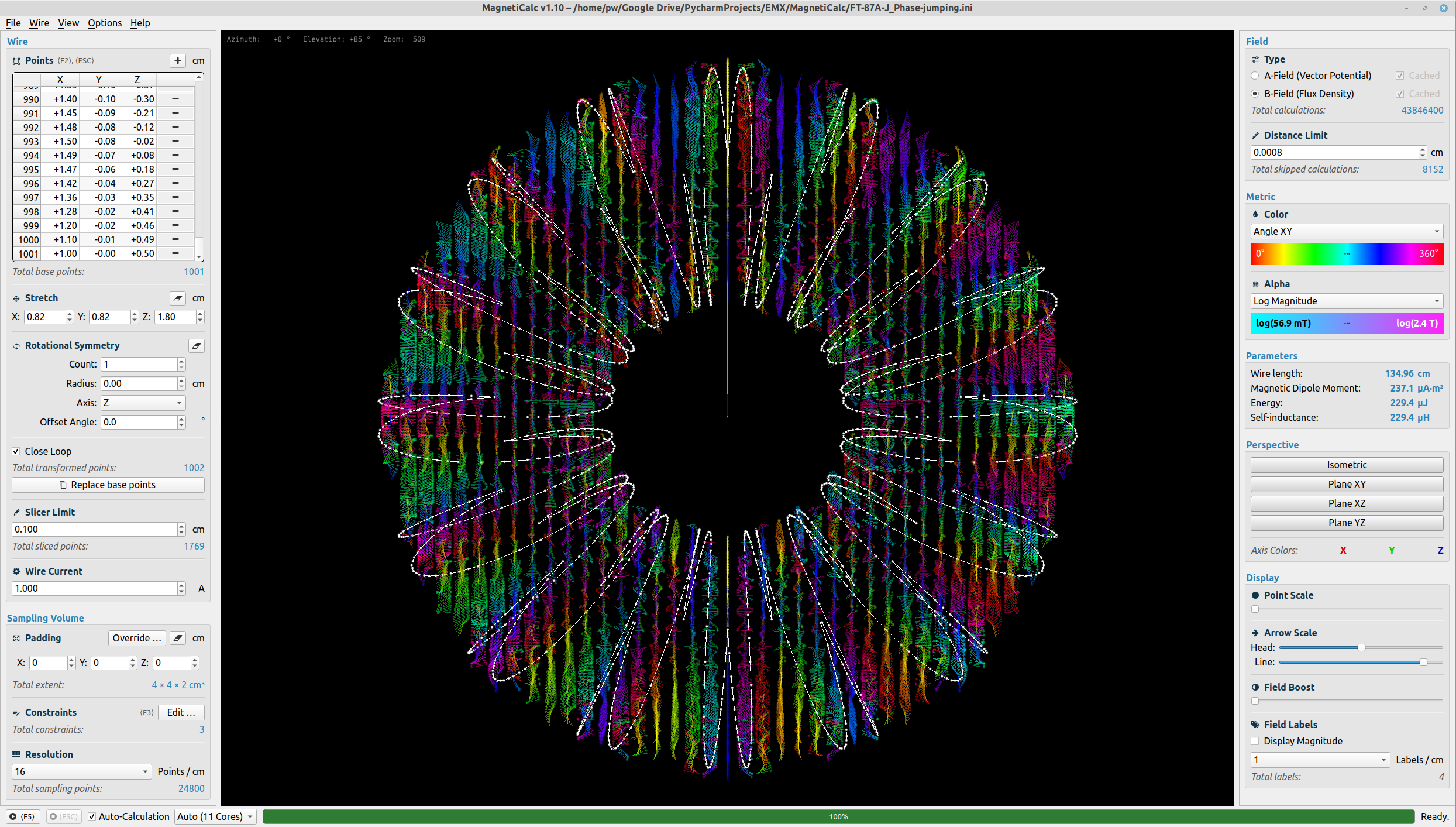
(Screenshot taken from the latest GitHub release.)

Examples

Some example projects can be found in the examples/ folder.

If you feel like your project should also be included as an example, you are welcome to file an issue!

Here’s the updated Installation section, drop-in ready and style-preserving:

Installation

If you have trouble installing MagnetiCalc, make sure to file an issue so I can help you get it up and running!

You can install MagnetiCalc either as a standard user or as a developer.

Requirements:

Python 3.9 … 3.12

Tested with:

Python 3.7 in Linux Mint 19.3
Python 3.8 in Ubuntu 20.04
Python 3.8.2 in macOS 11.6 (M1)
Python 3.8.10 in Windows 10 (21H2)
Python 3.10.5 in Ubuntu 20.04
Python 3.12.4 in Ubuntu 24.04

Important:

Linux users should reinstall the following driver to avoid errors like "Could not load the Qt platform plugin" : sudo apt install --reinstall libxcb-xinerama0

For Users

This is the recommended way to install MagnetiCalc if you just want to use it.

Install pipx

pipx is a tool that allows you to install and run Python applications in isolated environments. If you don't have it already, you can install it with:
```
sudo apt install pipx
```
Install MagnetiCalc
```
pipx install magneticalc
```
Run MagnetiCalc
```
magneticalc
```

For Developers

If you want to contribute to MagnetiCalc, you'll need to set up a development environment.

Install uv

uv is a fast Python package manager. Installation instructions: https://docs.astral.sh/uv/

Clone the repository

git clone https://github.com/shredEngineer/MagnetiCalc.git
cd MagnetiCalc

Install dependencies
```
uv sync
```
Run MagnetiCalc
```
uv run magneticalc
```

Enabling CUDA Support

Tested in Ubuntu 20.04, using the NVIDIA CUDA 10.1 driver and NVIDIA GeForce GTX 1650 GPU.

Please refer to the Numba Installation Guide which includes the steps necessary to get CUDA up and running.

License

ISC License

Permission to use, copy, modify, and/or distribute this software for any purpose with or without fee is hereby granted, provided that the above copyright notice and this permission notice appear in all copies.

THE SOFTWARE IS PROVIDED "AS IS" AND THE AUTHOR DISCLAIMS ALL WARRANTIES WITH REGARD TO THIS SOFTWARE INCLUDING ALL IMPLIED WARRANTIES OF MERCHANTABILITY AND FITNESS. IN NO EVENT SHALL THE AUTHOR BE LIABLE FOR ANY SPECIAL, DIRECT, INDIRECT, OR CONSEQUENTIAL DAMAGES OR ANY DAMAGES WHATSOEVER RESULTING FROM LOSS OF USE, DATA OR PROFITS, WHETHER IN AN ACTION OF CONTRACT, NEGLIGENCE OR OTHER TORTIOUS ACTION, ARISING OUT OF OR IN CONNECTION WITH THE USE OR PERFORMANCE OF THIS SOFTWARE.

Contribute

You are invited to contribute to MagnetiCalc!

General feedback, Issues and Pull Requests are always welcome.

If this software has been helpful to you in some way or another, please let me and others know!

Documentation

The documentation for MagnetiCalc is auto-generated from docstrings in the Python code.

Debugging

If desired, MagnetiCalc can be quite verbose about everything it is doing in the terminal:

Some modules are blacklisted in Debug.py, but this can easily be changed.
Some modules also provide their own debug switches to increase the level of detail.

Data Import/Export and Python API

GUI

MagnetiCalc allows the following data to be imported/exported using the GUI:

Import/export wire points from/to TXT file.
Export $\mathbf{A}$-/$\mathbf{B}$-fields, wire points and wire current to an HDF5 container for use in post-processing. Note: You could use Panoply to open HDF5 files. (The "official" HDFView software didn't work for me.)

API

The API class (documentation) provides basic functions for importing/exporting data programmatically.

Example: Wire Export

Generate a wire shape using NumPy and export it to a TXT file:

from magneticalc import API
import numpy as np

wire = [
    (np.cos(a), np.sin(a), np.sin(16 * a) / 5)
    for a in np.linspace(0, 2 * np.pi, 200)
]

API.export_wire("Custom Wire.txt", wire)

Example: Field Import

Import an HDF5 file containing an $\mathbf{A}$-field and plot it using Matplotlib:

from magneticalc import API
import matplotlib.pyplot as plt

data = API.import_hdf5("examples/Custom Export.hdf5")
axes = data.get_axes()
a_field = data.get_a_field()

ax = plt.figure

MagnetiCalc

Install / Use

README

MagnetiCalc

Screenshot

Examples

Installation

For Users

For Developers

Enabling CUDA Support

License

Contribute

Documentation

Debugging

Data Import/Export and Python API

GUI

API

Example: Wire Export

Example: Field Import