Lexcube

3D Data Cube Visualization in Jupyter Notebooks

---

GitHub: https://github.com/msoechting/lexcube

Paper: https://doi.org/10.1080/20964471.2025.2471646

PyPI: https://pypi.org/project/lexcube/

---

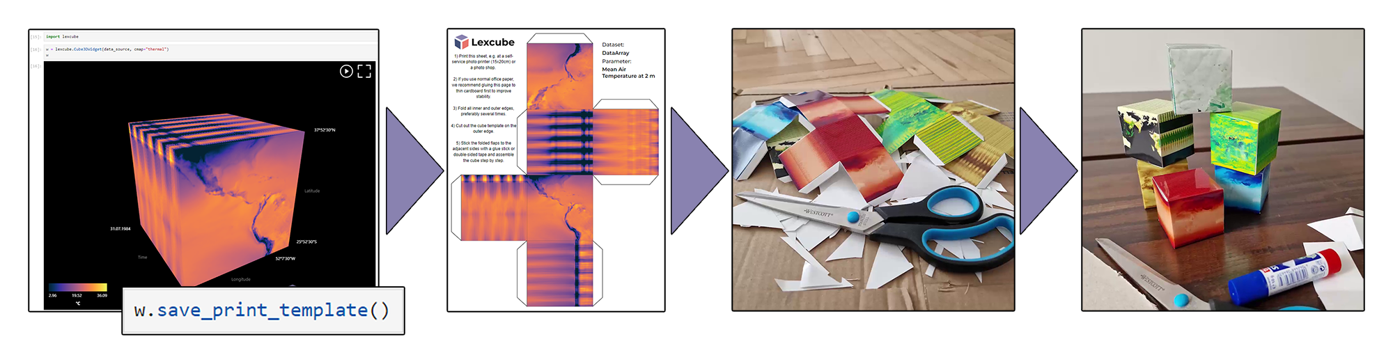
NEW with version 0.4.16: Craft your own paper data cube!

---

Lexcube is a library for interactively visualizing three-dimensional floating-point data as 3D cubes in Jupyter notebooks.

Supported data formats:

• numpy.ndarray (with exactly 3 dimensions)
• xarray.DataArray (with exactly 3 dimensions, rectangularly gridded)

Possible data sources:

• Any gridded Zarr or NetCDF data set (local or remote, e.g., accessed with S3)
• Copernicus Data Storage, e.g., ERA5 data
• Google Earth Engine (using xee, see example notebook)

Example notebooks can be found in the examples folder. For a live demo, see also lexcube.org.

Table-of-Contents

<!-- TOC tocDepth:2..3 chapterDepth:2..6 -->

• Table-of-Contents
• Attribution
• How to Use Lexcube
  • Example Notebooks
  • Getting Started - Minimal Example
    • Visualizing Xarray Data
    • Visualizing Numpy Data
    • Visualizing Google Earth Engine Data
    • Note on Google Collab
    • Note on Juypter for VSCode
• Installation
• Cube Visualization
• Interacting with the Cube
• Range Boundaries
• Colormaps
  • Supported colormaps
• Scaling the cube to fit your data
• Overlay GeoJSON data
• Save figures
• Saving camera angles & reproducing figures
• Print your own paper data cube
• Get currently visible data subset
• Supported metadata
• Troubleshooting
  • The cube does not respond / API methods are not doing anything / Cube does not load new data
  • After installation/update, no widget is shown, only text
  • w.savefig breaks when batch-processing/trying to create many figures quickly
  • The layout of the widget looks very messed up
  • "Error creating WebGL context" or similar
  • Memory is filling up a lot when using a chunked dataset
• Known bugs
• Attributions
• Development Installation & Guide
• License

<!-- /TOC -->

Attribution

When using Lexcube and generated images or videos, please acknowledge/cite:

@article{Soechting2025Lexcube,
    author = {Maximilian Söchting and Gerik Scheuermann and David Montero and Miguel D. Mahecha},
    title = {Interactive Earth system data cube visualization in Jupyter notebooks},
    journal = {Big Earth Data},
    pages = {1--15},
    year = {2025},
    publisher = {Taylor \& Francis},
    doi = {10.1080/20964471.2025.2471646},
    URL = {https://doi.org/10.1080/20964471.2025.2471646},
}

Lexcube is a project by Maximilian Söchting at the RSC4Earth at Leipzig University, advised by Prof. Dr. Miguel D. Mahecha and Prof. Dr. Gerik Scheuermann. Thanks to the funding provided by ESA through DeepESDL and DFG through the NFDI4Earth pilot projects!

How to Use Lexcube

Example Notebooks

If you are new to Lexcube, try the general introduction notebook which demonstrates how to visualize a remote Xarray data set.

There are also specific example notebooks for the following use cases:

• Visualizing Google Earth Engine data - using xee
• Generating and visualizing a spectral index data cube from scratch - using cubo and spyndex, with data from Microsoft Planetary Computer
• Generating and visualizing a spectral index data cube - with data from OpenEO
• Visualizing Numpy data

Getting Started - Minimal Example

Visualizing Xarray Data

import xarray as xr
import lexcube 
ds = xr.open_dataset("https://data.rsc4earth.de/download/EarthSystemDataCube/v3.0.2/esdc-8d-0.25deg-256x128x128-3.0.2.zarr/", chunks={}, engine="zarr")
da = ds["air_temperature_2m"][256:512,256:512,256:512]
w = lexcube.Cube3DWidget(da, cmap="thermal_r", vmin=-20, vmax=30)
w.plot()

Visualizing Numpy Data

import numpy as np
import lexcube 
data_source = np.sum(np.mgrid[0:256,0:256,0:256], axis=0)
w = lexcube.Cube3DWidget(data_source, cmap="prism", vmin=0, vmax=768)
w.plot()

Visualizing Google Earth Engine Data

See the full example here.

import lexcube
import xarray as xr
import ee
ee.Authenticate()
ee.Initialize(opt_url="https://earthengine-highvolume.googleapis.com")
ds = xr.open_dataset("ee://ECMWF/ERA5_LAND/HOURLY", engine="ee", crs="EPSG:4326", scale=0.25, chunks={})
da = ds["temperature_2m"][630000:630003,2:1438,2:718]
w = lexcube.Cube3DWidget(da)
w.plot()

Note on Google Collab

If you are using Google collab, you may need to execute the following before running Lexcube:

from google.colab import output
output.enable_custom_widget_manager()

Note on Juypter for VSCode

If you are using Jupyter within VSCode, you may have to add the following to your settings before running Lexcube:

    "jupyter.widgetScriptSources": [
        "jsdelivr.com",
        "unpkg.com"
    ],

If you are working on a remote server in VSCode, do not forget to set this setting also there! This allows the Lexcube JavaScript front-end files to be downloaded from these sources (read more).

Installation

You can install using pip:

pip install lexcube

After installing or upgrading Lexcube, you should refresh the Juypter web page (if currently open) and restart the kernel (if currently running).

If you are using Jupyter Notebook 5.2 or earlier, you may also need to enable the nbextension:

jupyter nbextension enable --py [--sys-prefix|--user|--system] lexcube

Cube Visualization

On the cube, the dimensions are visualized as follow: X from left-to-right (0 to max), Y from top-to-bottom (0 to max), Z from back-to-front (0 to max); with Z being the first dimension (axis[0]), Y the second dimension (axis[1]) and X the third dimension (axis[2]) on the input data. If you prefer to flip any dimension or re-order dimensions, you can modify your data set accordingly before calling the Lexcube widget, e.g. re-ordering dimensions with xarray: ds.transpose(ds.dims[0], ds.dims[2], ds.dims[1]) and flipping dimensions with numpy: np.flip(ds, axis=1).

Interacting with the Cube

• Zooming in/out on any side of the cube:
  • Mousewheel
  • Scroll gesture on touchpad (two fingers up or down)
  • On touch devices: Two-touch pinch gesture
• Panning the currently visible selection:
  • Click and drag the mouse cursor
  • On touch devices: touch and drag
• Moving over the cube with your cursor will show a tooltip in the bottom left about the pixel under the cursor.
• For more precise input, you can use the sliders provided by w.show_sliders():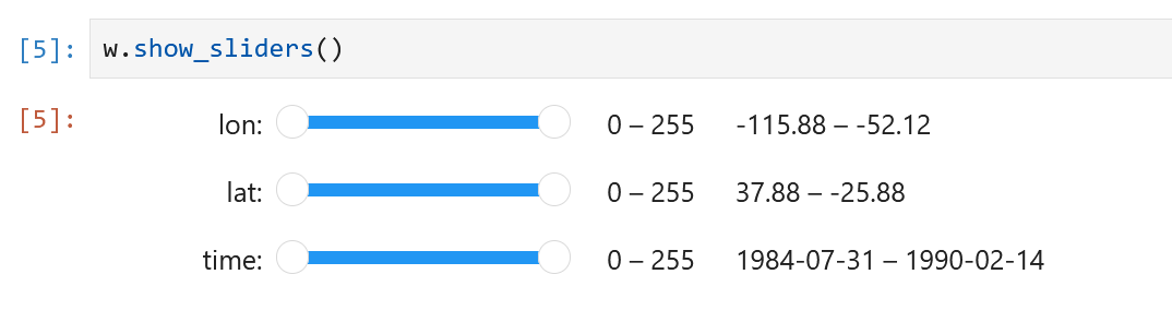

Range Boundaries

You can read and write the boundaries of the current selection via the xlim, ylim and zlim tuples.

w = lexcube.Cube3DWidget(da, cmap="thermal", vmin=-20, vmax=30)
w.plot()
# Next cell:
w.xlim = (20, 400)

For fine-grained interactive controls, you can display a set of sliders in another cell, like this:

w = lexcube.Cube3DWidget(da, cmap="thermal", vmin=-20, vmax=30)
w.plot()
# Next cell:
w.show_sliders()

For very large data sets, you may want to use w.show_sliders(continuous_update=False) to prevent any data being loaded before making a final slider selection.

If you want to wrap around a dimension, i.e., seamleasly scroll over back to the 0-index beyond the maximum index, you can enable that feature like this: