<img src="https://github.com/kharchenkolab/conos/blob/dev/inst/conos_logo.png" align="right" height="140">

conos

• Introduction
• Basics of using conos
• Tutorials
  • Conos walkthrough
  • Adjustment of alignment strength with conos
  • Integration with Scanpy
  • Integrating RNA-seq and ATAC-seq with conos
  • Running RNA velocity on a Conos object
• Installation
  • Running conos via Docker
• References

Conos: Clustering On Network Of Samples

• What is conos? Conos is an R package to wire together large collections of single-cell RNA-seq datasets, which allows for both the identification of recurrent cell clusters and the propagation of information between datasets in multi-sample or atlas-scale collections. It focuses on the uniform mapping of homologous cell types across heterogeneous sample collections. For instance, users could investigate a collection of dozens of peripheral blood samples from cancer patients combined with dozens of controls, which perhaps includes samples of a related tissue such as lymph nodes.

• How does it work? 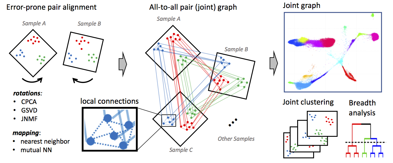Conos applies one of many error-prone methods to align each pair of samples in a collection, establishing weighted inter-sample cell-to-cell links. The resulting joint graph can then be analyzed to identify subpopulations across different samples. Cells of the same type will tend to map to each other across many such pairwise comparisons, forming cliques that can be recognized as clusters (graph communities).

  Conos processing can be divided into three phases:

  • Phase 1: Filtering and normalization Each individual dataset in the sample panel is filtered and normalized using standard packages for single-dataset processing: either pagoda2 or Seurat. Specifically, Conos relies on these methods to perform cell filtering, library size normalization, identification of overdispersed genes and, in the case of pagoda2, variance normalization. (Conos is robust to variations in the normalization procedures, but it is recommended that all of the datasets be processed uniformly.)
  • Phase 2: Identify multiple plausible inter-sample mappings Conos performs pairwise comparisons of the datasets in the panel to establish an initial error-prone mapping between cells of different datasets.
  • Phase 3: Joint graph construction These inter-sample edges from Phase 2 are then combined with lower-weight intra-sample edges during the joint graph construction. The joint graph is then used for downstream analysis, including community detection and label propagation. For a comprehensive description of the algorithm, please refer to our publication.

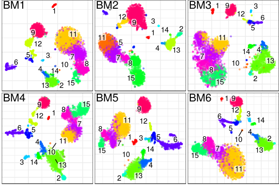
• What does it produce? In essence, conos will take a large, potentially heterogeneous panel of samples and will produce clustering grouping similar cell subpopulations together in a way that will be robust to inter-sample variation:
  

• What are the advantages over existing alignment methods? Conos is robust to heterogeneity of samples within a collection, as well as noise. The ability to resolve finer subpopulation structure improves as the size of the panel increases.

Basics of using conos

Given a list of individual processed samples (pl), conos processing can be as simple as this:

# Construct Conos object, where pl is a list of pagoda2 objects 
con <- Conos$new(pl)

# Build joint graph
con$buildGraph()

# Find communities
con$findCommunities()

# Generate embedding
con$embedGraph()

# Plot joint graph
con$plotGraph()

# Plot panel with joint clustering results
con$plotPanel()

To see more documentation on the class Conos, run ?Conos.

Tutorials

Please see the following tutorials for detailed examples of how to use conos:

Conos walkthrough:

• HTML version
• Markdown version

Adjustment of alignment strength with conos:

• HTML version
• Markdown version

Integration with Scanpy:

Note that for integration with Scanpy, users need to save conos files to disk from an R session, and then load these files into Python.

Save conos for Scanpy:

• HTML version
• Markdown version

Load conos files into Scanpy:

• Jupyter Notebook

Integrating RNA-seq and ATAC-seq with conos:

• HTML version
• Markdown version

Running RNA velocity on a Conos object

First of all, in order to obtain an RNA velocity plot from a Conos object you have to use the dropEst pipeline to align and annotate your single-cell RNA-seq measurements. You can see this tutorial and this shell script to see how it can be done. In this example we specifically assume that when running dropEst you have used the -V option to get estimates of unspliced/spliced counts from the dropEst directly. Secondly, you need the velocyto.R package for the actual velocity estimation and visualisation.

After running dropEst you should have 2 files for each of the samples:

• sample.rds (matrix of counts)
• sample.matrices.rds (3 matrices of exons, introns and spanning reads)

The .matrices.rds files are the velocity files. Load them into R in a list (same order as you give to conos). Load, preprocess and integrate with conos the count matrices (.rds) as you normally would. Before running the velocity, you must at least create an embedding and run the leiden clustering. Finally, you can estimate the velocity as follows:

### Assuming con is your Conos object and cms.list is the list of your velocity files ###

library(velocyto.R)

# Preprocess the velocity files to match the Conos object
vi <- velocityInfoConos(cms.list = cms.list, con = con, 
                        n.odgenes = 2e3, verbose = TRUE)

# Estimate RNA velocity
vel.info <- vi %$%
  gene.relative.velocity.estimates(emat, nmat, cell.dist = cell.dist, 
                                   deltaT = 1, kCells = 25, fit.quantile = 0.05, n.cores = 4)

# Visualise the velocity on your Conos embedding 
# Takes a very long time! 
# Assign to a variable to speed up subsequent recalculations
cc.velo <- show.velocity.on.embedding.cor(vi$emb, vel.info, n = 200, scale = 'sqrt', 
                                          cell.colors = ac(vi$cell.colors, alpha = 0.5), 
                                          cex = 0.8, grid.n = 50, cell.border.alpha = 0,
                                          arrow.scale = 3, arrow.lwd = 0.6, n.cores = 4, 
                                          xlab = "UMAP1", ylab = "UMAP2")

# Use cc=cc.velo$cc when running again (skips the most time consuming delta projections step)
show.velocity.on.embedding.cor(vi$emb, vel.info, cc = cc.velo$cc, n = 200, scale = 'sqrt', 
                               cell.colors = ac(vi$cell.colors, alpha = 0.5), 
                               cex = 0.8, arrow.scale = 15, show.grid.flow = TRUE, 
                               min.grid.cell.mass = 0.5, grid.n = 40, arrow.lwd = 2,
                               do.par = F, cell.border.alpha = 0.1, n.cores = 4,
                               xlab = "UMAP1", ylab = "UMAP2")

Installation

To install the stable version from CRAN, use:

install.packages('conos')

To install the latest version of conos, use:

install.packages('devtools')
devtools::install_github('kharchenkolab/conos')

System dependencies

The dependencies are inherited from pagoda2. Note that this package also has the dependency igraph, which requires various libraries to install correctly. Please see the installation instructions at that page for more details, along with the github README here.

Ubuntu dependencies

To install system dependencies using apt-get, use the following:

sudo apt-get update
sudo apt-get -y install libcurl4-openssl-dev libssl-dev libxml2-dev libgmp-dev libglpk-dev

Red Hat-based distributions dependencies

For Red Hat distributions using yum, use the following command:

sudo yum update
sudo