<p align="center"> <img src="https://github.com/ADCMEMarket/ADCMEImages/blob/master/ADCME/ADCME.gif?raw=true" alt="ADCME"/> </p>

The ADCME library (Automatic Differentiation Library for Computational and Mathematical Engineering) aims at general and scalable inverse modeling in scientific computing with gradient-based optimization techniques. It is built on the deep learning framework, graph-mode TensorFlow, which provides the automatic differentiation and parallel computing backend. The dataflow model adopted by the framework makes it suitable for high performance computing and inverse modeling in scientific computing. The design principles and methodologies are summarized in the slides.

Check out more about slides and videos on ADCME!

| Install ADCME and Get Started (Windows, Mac, and Linux) | Scientific Machine Learning for Inverse Modeling | Solving Inverse Modeling Problems with ADCME | ...more on ADCME Youtube Channel! | | ------------------------------------------------------------ | ------------------------------------------------------------ | ------------------------------------------------------------ | ------------------------------------------------------------ | | | | | |

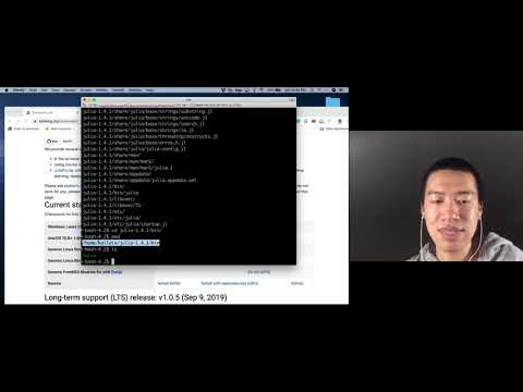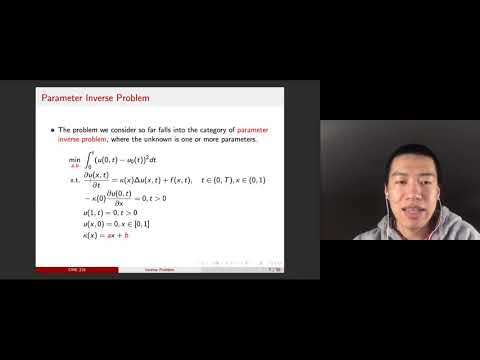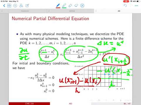Several features of the library are

• MATLAB-style Syntax. Write A*B for matrix production instead of tf.matmul(A,B).
• Custom Operators. Implement operators in C/C++ for performance critical parts; incorporate legacy code or specially designed C/C++ code in ADCME; automatic differentiation through implicit schemes and iterative solvers.
• Numerical Scheme. Easy to implement numerical schemes for solving PDEs.
• Physics Constrained Learning. Embed neural network into PDEs and solve with any numerical schemes, including implicit and iterative schemes.
• Static Graphs. Compilation time computational graph optimization; automatic parallelism for your simulation codes.
• Parallel Computing. Concurrent execution and model/data parallel distributed optimization.
• Custom Optimizers. Large scale constrained optimization? Use CustomOptimizer to integrate your favorite optimizer. Try out prebuilt Ipopt and NLopt optimizers.
• Sparse Linear Algebra. Sparse linear algebra library tailored for scientific computing.
• Inverse Modeling. Many inverse modeling algorithms have been developed and implemented in ADCME, with wide applications in solid mechanics, fluid dynamics, geophysics, and stochastic processes.
• Finite Element Method. Get AdFem.jl today for finite element simulation and inverse modeling!

Start building your forward and inverse modeling using ADCME today!

| Documentation | Tutorial | Applications | | ------------------------------------------------------------ | ------------------------------------------------------------ | ------------------------------------------------------------ | | | | |

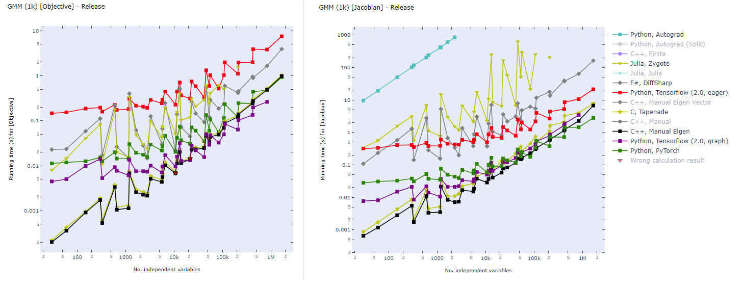
Graph-mode TensorFlow for High Performance Scientific Computing

Static computational graph (graph-mode AD) enables compilation time optimization. Below is a benchmark of common AD software from here. In inverse modeling, we usually have a scalar-valued objective function, so the left panel is most relevant for ADCME.

Installation

1. Install Julia.

🎉 Support Matrix

| | Julia≧1.3 | GPU | Custom Operator | |---------| ----- |-----|-----------------| | Linux |✔ | ✔ | ✔ | | MacOS |✔ | ✕ | ✔ | | Windows | ✔ | ✔ | ✔ |

1. Install ADCME

using Pkg
Pkg.add("ADCME")

❗ FOR WINDOWS USERS: See the instruction or the video for installation details.

❗ FOR MACOS USERS: See this troubleshooting list for potential installation and compilation problems on Mac.

2. (Optional) Test ADCME.jl

using Pkg
Pkg.test("ADCME")

See Troubleshooting if you encounter any compilation problems.

3. (Optional) To enable GPU support, make sure nvcc is available from your environment (e.g., type nvcc in your shell and you should get the location of the executable binary file), and then type

ENV["GPU"] = 1
Pkg.build("ADCME")

You can check the status with using ADCME; gpu_info().

4. (Optional) Check the health of your installed ADCME and install missing dependencies or fixing incorrect paths.

using ADCME 
doctor()

For manual installation without access to the internet, see here.

Install via Docker

If you have Docker installed on your system, you can try the no-hassle way to install ADCME (you don't even have to install Julia!):

docker run -ti kailaix/adcme

For GPU-enabled ADCME, use

docker run -ti --gpus all kailaix/adcme:gpu

See this guide for details. The docker images are hosted here.

Tutorial

Here we present three inverse problem examples. The first one is a parameter estimation problem, the second one is a function inverse problem where the unknown function does not depend on the state variables, and the third one is also a function inverse problem, but the unknown function depends on the state variables.

Parameter Inverse Problem

Consider solving the following problem

where

Assume that we have observed u(0.5)=1, we want to estimate b. In this case, he true value should be b=1.

using LinearAlgebra
using ADCME

n = 101 # number of grid nodes in [0,1]
h = 1/(n-1)
x = LinRange(0,1,n)[2:end-1]

b = Variable(10.0) # we use Variable keyword to mark the unknowns
A = diagm(0=>2/h^2*ones(n-2), -1=>-1/h^2*ones(n-3), 1=>-1/h^2*ones(n-3)) 
B = b*A + I  # I stands for the identity matrix
f = @. 4*(2 + x - x^2) 
u = B\f # solve the equation using built-in linear solver
ue = u[div(n+1,2)] # extract values at x=0.5

loss = (ue-1.0)^2 

# Optimization
sess = Session(); init(sess) 
BFGS!(sess, loss)

println("Estimated b = ", run(sess, b))

Expected output

Estimated b = 0.9995582304494237

The gradients can be obtained very easily. For example, if we want the gradients of loss with respect to b, the following code will create a Tensor for the gradient

julia> gradients(loss, b)
PyObject <tf.Tensor 'gradients_1/Mul_grad/Reshape:0' shape=() dtype=float64>

Function Inverse Problem: Full Field Data

Consider a nonlinear PDE,

where

Here f(x) can be computed from an analytical solution

In this problem, we are given the full field data of u(x) (the discrete value of u(x) is given on a very fine grid) and want to estimate the nonparametric function b(u). We approximate b(u) using a neural network and use the residual minimization method to find the optimal weig