Deferred Voxel Shading for Real Time Global Illumination

Overview
Results
Executable

Peer-review published paper for this technique can be found here:

https://github.com/jose-villegas/VCTRenderer/blob/master/paper_final.pdf http://ieeexplore.ieee.org/abstract/document/7833375/

The thesis can be found here (Spanish) here: https://raw.githubusercontent.com/jose-villegas/ThesisDocument/master/Tesis.pdf

Computing indirect illumination is a challenging and complex problem for real-time rendering in 3D applications. This global illumination approach computes indirect lighting in real time utilizing a simpliﬁed version of the outgoing radiance and the scene stored in voxels.

Overview

Deferred voxel shading is a four-step real-time global illumination technique inspired by voxel cone tracing and deferred rendering. This approach enables us to obtain an accurate approximation of a plethora of indirect illumination effects including: indirect diffuse, specular reflectance, color-blending, emissive materials, indirect shadows and ambient occlusion. The steps that comprehend this technique are described below.

<table> <tr> <th>Technique Overview</th> </tr> <tr> <td align="center"><img src="https://res.cloudinary.com/jose-villegas/image/upload/v1738340934/template_primary_k4ezzu.jpg" style="width: 100%; background-color: #cccccc;"/></td> </tr> </table>

1. Voxelization

The first step is to voxelize the scene, our implemention voxelizes scene albedo, normal and emission to approximate emissive materials. For this conservative voxelization and atomic operations on 3D textures are used as described here.

...
layout(binding = 0, r32ui) uniform volatile coherent uimage3D voxelAlbedo;
layout(binding = 1, r32ui) uniform volatile coherent uimage3D voxelNormal;
layout(binding = 2, r32ui) uniform volatile coherent uimage3D voxelEmission;
...
// average normal per fragments sorrounding the voxel volume
imageAtomicRGBA8Avg(voxelNormal, position, normal);
// average albedo per fragments sorrounding the voxel volume
imageAtomicRGBA8Avg(voxelAlbedo, position, albedo);
// average emission per fragments sorrounding the voxel volume
imageAtomicRGBA8Avg(voxelEmission, position, emissive);
...

| Scene | Average Albedo | Average Normal | Average Emission | |-------|----------------|----------------|------------------| <img src="http://res.cloudinary.com/jose-villegas/image/upload/v1497323827/DVSGI/scene_culelk.png" style="width: 100%;"/>|<img src="http://res.cloudinary.com/jose-villegas/image/upload/v1497323820/DVSGI/v_albedo_qtc4ov.png" style="width: 100%;"/>|<img src="http://res.cloudinary.com/jose-villegas/image/upload/v1497323804/DVSGI/v_normal_ryzmrh.png" style="width: 100%;"/>|<img src="http://res.cloudinary.com/jose-villegas/image/upload/v1497323828/DVSGI/v_emission_aibyaf.png" style="width: 100%;"/>

1.1. Voxel Structure

The voxel structure is inspired by deferred rendering, where a G-Buffer contains relevant data to later be used in a separate light pass. Normal, albedo and emission values are stored in voxels during the voxelization process, every attribute has its own 3D texture associated. This information is sufficient to calculate the diffuse reflectance and normal attenuation on a separate light pass where, instead of computing the lighting per pixel it is done per voxel. The structure can be extended to support a more complicated reflectance model but this may imply a higher memory consumption to store additional data.

Furthermore, another structure is used for the voxel cone tracing pass. The resulting values of the lighting computations per voxel are stored in another 3D texture which we will call radiance volume. To approximate the incrementing diameter of the cone, and its sampling volume, levels of detail of the voxelized scene are used. For anisotropic voxels six 3D textures at half resolution of the radiance volume are required, one per every axis direction positive and negative, the levels of details are stored within the mipmap levels of these textures which we will call directional volumes.

The radiance volume represents the maximum level of detail for the voxelized scene, this texture is separated from the directional volumes. To bind these two structures, linear interpolation is used between samples of both structures when the mipmap level required for the diameter of the cone ranges between, the maximum level and the first filtered level of detail.

<table> <tr> <th>A visualization of the voxel structure</th> </tr> <tr> <td align="center"><img src="https://res.cloudinary.com/jose-villegas/image/upload/v1738337277/vegllzlmgdmns9exq1hp.svg" style="width: 100%;"/></td> </tr> </table>

1.2. Dynamic Voxelization

For dynamic updates, the conservative voxelization of static and dynamic geometry are separated. While static voxelization happens only once, dynamic voxelization happens per frame or when needed. The voxelization for both types of geometry rely on the same process, hence a way to indicate which voxels are static is needed. In our approach we use a single value 3D texture to identify voxels as static, this texture will be called flag volume.

During static voxelization, after a voxel is generated a value is written to the flag volume indicating this position as static. In contrast, during the dynamic voxelization, before generating a voxel, a value is read from the flag volume at the writing position of the voxel, if the value indicates this position is marked as static then writing is discarded, leaving the static voxels untouched.

To constantly revoxelize the scene it is necessary to clear from the 3D textures the previous stored dynamic voxels. This is done before the dynamic voxelization using compute shaders. The flag volume is read to clear voxels under two conditions: if the voxel exists and if it’s dynamic.

2. Voxel Illumination

The second step is voxel illumination, for this we calculate the outgoing radiance per voxel using the data stored from the voxelization step. For this we only need the voxel normal, and its position which can be easily extracted by projecting the voxel 3D coordinates in world-space, then we can calculate the direct lighting per voxel. This is all done in a compute shader.

One of the advantages of this technique is that it's compatible with all standard light types like point, spot and directional lights, another is that we don't need shadow maps, though they can help greatly with precision specially for directional lights. Other techniques calculate the voxel radiance per light's shadow map, meaning that for every shadow-mapped light that wants to contribute to the voxel radiance the illumination step has to be repeated.

| Scene | Voxel Direct Lighting | |:-----:|:---------------------:| <img src="http://res.cloudinary.com/jose-villegas/image/upload/v1497323827/DVSGI/scene_culelk.png" style="width: 100%"/>|<img src="http://res.cloudinary.com/jose-villegas/image/upload/v1497323829/DVSGI/v_direct_vrnajc.png" style="width: 100%"/>

2.1. Normal-Weighted Attenuation

A disvantage of this technique is the loss of precision averaging all the geometry normals within a voxel. The resulting averaged normal may end up pointing towards a non-convenient direction. This problem is notable when the normal vectors within the space of a voxel are uneven:

</center>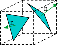

To reduce this issue our proposal utilizes a normal-weighted attenuation, where first the normal attenuation is calculated per every face of the voxel as follows:

Then three dominant faces are selected depending on the axes sign of the voxel averaged normal vector:

<img src="https://latex.codecogs.com/png.image?\inline&space;\LARGE&space;\dpi{110}\bg{white}D_{\omega}=\begin{cases}max\{D_{\omega},0\},&N_{\omega}>0\\max\{-D_{\omega},0\},&\text{otherwise}\end{cases}" title="D_{\omega}=\begin{cases}max\{D_{\omega},0\},&N_{\omega}>0\\max\{-D_{\omega},0\},&\text{otherwise}\end{cases}" />

And finally, the resulting attenuation is the product of every dominant face normal attenuation, multiplied with the weight per axis of the averaged normal vector of the voxel, the r

VCTRenderer

Install / Use

README