quantfinance

This work was developed together with my former university colleagues for a financial engineering project. I thank Claudio Ragaglia, Marco Lombardi, Davide Furnò, Carmelo Pepe and Giacomo Abramo for this great job!

Our project aims to analyze and obtain an options investment strategy, having the Oil Futures (WTI Crude Oil) as underlying. The analysis is based on a Monte Carlo simulation that takes the historical data of the underlying from Yahoo Finance; it calculates its historical volatility and indicates its latest price (May 9, 2020). On the basis of the prices, the risk free rate and the maturity taken as reference (17 June 2020), it carries out “i” simulations, for a predetermined number of steps, estimating the average price at maturity. After running the Monte Carlo simulation, through the Black-Scholes-Merton model, we calculate the price of the options with the data of May 9, 2020. We also present an alternative calculation through the Black model (which are almost equal). Once the prices of the options have been calculated, we have evaluated which strategy to implement based on the options available on the market. We therefore opted for a Put Spread Ratio strategy which consists of buying a Put with a strike price of 30 and shorting 2 Put with a strike price of 25. Then we have the profit positions of the individual options, reaching the graphic screen of the strategy and indicating the maximum payoffs and minimums. Finally, we concluded with the calculation of the Greek and the respective plots. We also present part of the project using an open source library, QuantLib.

Monte Carlo model for forecasting the underlying.

In this phase we will use the Monte Carlo model to forecast the price of Crude Oil at the expiry of the option, on 17/06/2020. We have defined the time period T to be used for the calculation of historical volatility as the period from 01/04/2020 to 09/05/2020, i.e. the same time period (39 days) that there are from the valuation date (09/05/2020) upon expiry of the contract (17/6/2020). Next, we calculated the volatility (by directly importing the price of the underlying from Yahoo Finance), obtaining the value of 0.2857057186685205. For the risk-free interest rate we used 10 Years Treasury Yield (^ TNX), as a proxy, thus obtaining the value of 0.068. We decided to use 100 steps for the simulation and 1000 simulations. From the Monte Carlo model we obtained the following graph:

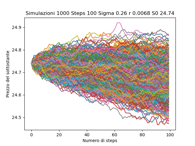
With the following expected price of Crude Oil as of 06/17/2020: 24.561763286859474.

Black & Scholes

After obtaining an estimate of the future price of the underlying, in order to build and analyze our strategy we need the prices of the options, so we used the Black & Scholes formula to price them. We know that the Black & Scholes formula is as follows:

<img src="https://render.githubusercontent.com/render/math?math={\color{white} c = S_0 N(d_1) \%2d K e^{-rt} N(d_2)}"> <img src="https://render.githubusercontent.com/render/math?math={\color{white} c = K e^{-rt} N(\%2d d_2) \%2d S_0 N(\%2d d_1) }">

where,

<img src="https://render.githubusercontent.com/render/math?math={\color{white} d_1 = \dfrac{\ln(S_0/K) \%2b (r \%2b \sigma^2 / 2) T } {\sigma \sqrt{T}}}"> <img src="https://render.githubusercontent.com/render/math?math={\color{white} d_2 = \dfrac{\ln(S_0/K) \%2b (r \%2d \sigma^2 / 2) T } {\sigma \sqrt{T}} = d_1 \%2d \sigma \sqrt{T}}">

The inputs used to price the options are as follows:

• The value of the underlying (S) on the valuation date (09/05/2020) is 24,629 (Yahoo Finance, Crude Oil, code CL = F);
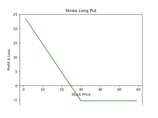
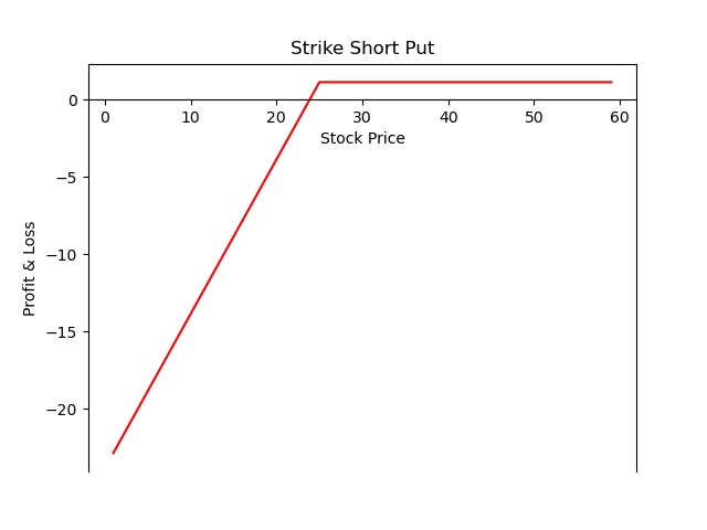
• The strike price (K) of the two puts is respectively $ 25 for the two short Put and $ 30 for the long Put (source: Barchart);
• The time (T) is 39 days, which are exactly the days from the valuation date to the expiry date of the option (17/06/2020);
• The volatility (sigma) is 0.2857 (historical volatility calculated previously);
• Finally, the risk-free (rf) rate is 0.0068 (we used 10 Years Treasury Yield (^ TNX), as a proxy of the rate); The results obtained are:
• The Higher_Long_Put by Black & Scholes Price is 5.3658, which therefore indicates the price of the Put we want to buy;
• The Lower_Short_Put by Black & Scholes Price is 1.1171, which instead indicates the price of the Put we want to sell. We will use these values ​​in the next steps for defining and evaluating the strategy. An alternative to the Black & Scholes formula for the valuation of European options is the model by Black, which we used to price the same options and evaluate the differences. The formula of Black's model is:

<img src="https://render.githubusercontent.com/render/math?math={\color{white} c = e^{-rT} [F_0 N(d_1) \%2d K N(d_2)]}"> <img src="https://render.githubusercontent.com/render/math?math={\color{white} p = e^{-rT} [K N(d_2) \%2d F_0 N(d_1)]}">

where,

<img src="https://render.githubusercontent.com/render/math?math={\color{white} d_1 = \dfrac{\ln(F_0 / K) \%2b (r \%2b \sigma^2 / 2) T } {\sigma \sqrt{T}}}"> <img src="https://render.githubusercontent.com/render/math?math={\color{white} d_2 = \dfrac{\ln(F_0/K) \%2d ( \sigma^2 / 2) T } {\sigma \sqrt{T}} = d_1 \%2d \sigma \sqrt{T}}">

The inputs are the same and after implementing it in Python, the results are:

• The Higher_Long_Put by Black Price is 5.3836, which therefore indicates the price of the Put we want to buy;
• The Lower_Short_Put by Black Price is 1.1269, which instead indicates the price of the Put we want to sell. If we compare the results we understand that in this case the values obtained are not very different.

Put Spread Ratio

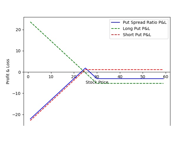
After identifying the options on the market with expiration on May 9, 2020, an investment strategy was assessed. After some tests, given the small number of options available on the market, it was decided to adopt a Put Spread Ratio Strategy with a ratio of 1 to 2. The options selected are the Put with strike price 30 and the Put with strike price 25, whose prices were determined in the previous paragraph. The strategy implemented specifically provides for the purchase of the first for one unit and the sale of the second for two units.

The form taken by the strategy is as follows:

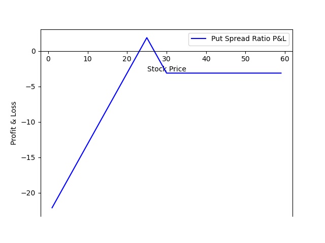
The strategy, if the forecasts on the underlying are correct, would allow us to achieve, at maturity, a profit very close to the maximum potential, which is equal to 1.87 points.

We also present the summary chart:

Evaluation of the strategy by using the Greeks

Through the use of the Greek it was possible to find various measures of the risk associated with the possession of one or more options. The first Greek used is the Delta, whose formula is expressed as follows:

<img src="https://render.githubusercontent.com/render/math?math={\color{white} \Delta = \dfrac{\delta P}{\delta S_0} }">

P = premium of the put option 𝑆0 = price of the underlying at period t0

This Greek defines the marginal variation of the Put price to the marginal variation of the underlying. In general, the Delta of a long Put option is negative, while for short Put options it will be positive. This result will give a positive measure of our Delta together with the Put Spread Ratio strategy.

Delta strategy: 0.10347088962020612

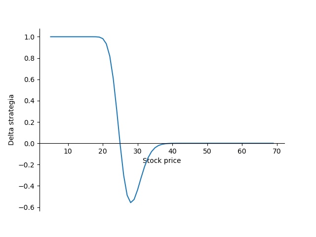
Correspondingly when Delta is equal to 1, as a point of the stock price changes, the strategy varies in a unitary manner (very sensitive up to the stock price value of 20). Subsequently, the strategy premium becomes less and less sensitive to the change in the price of the underlying, until it becomes indifferent to stock price 25; subsequently it becomes negative up to stock price 35 and then becomes indifferent up to stock price 69. The second Greek used is Gamma whose expression is given by:

<img src="https://render.githubusercontent.com/render/math?math={\color{white} \Theta = \dfrac{\delta^2P}{\delta S^2}}">

The range of a derivative portfolio is the derivative of the portfolio's Delta with respect to the price of the underlying asset. If the Gamma is small the Delta changes very slowly and the adjustments, to maintain risk neutrality in terms of Delta, do not need to be made frequently. If the Gamma is large in absolute terms, the Delta is very sensitive to the change in the price of the underlying asset.

The fretboard at strike values 25 and 30 assumes maximum absolute values.

Gamma strategy -0.3212757738004029

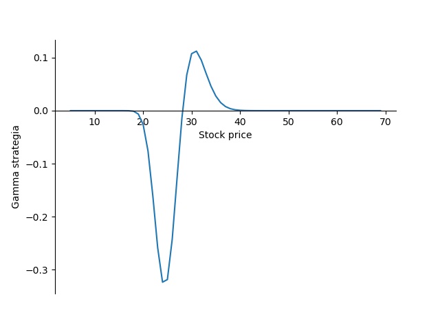
In general, Gamma has a trend that depends on the Delta (being the second derivative of the same). When Delta is constant, Gamma will be equal to 0. The value of Gamma with respect to the variation of the stock price tends to decrease during the decrease of Delta; as the stock price increases, Gamma increases dramatically; at the Delta inflection point, Gamma zeroes out. The third Greek used is Theta whose formula is the following:

<img src="https://render.githubusercontent.com/render/math?math={\color{white} \Omega = \dfrac{\delta pi}{\delta t}}">

The Theta of an options portfolio is the derivative of the portfolio's value over time.

Theta measures the change in the value of the portfolio as a result of the passage of an instant of time. It is almost always negative, since as the r