IFCshiny

<!-- badges: start --> <!--[](https://github.com/gitdemont/IFCshiny/actions) --> <!-- badges: end -->

An R Interactive Shiny Application for the Analysis of Imaging and Conventional Flow Cytometry (IFCshiny)

INSTALLATION (from in-dev github master branch)

IFCshiny package is under development and can be installed from github

On Windows (tested 7 and 10)

• install Rtools for windows

• ensure that Rtools compiler is present in Windows PATH

In R console, if you installed Rtools directly on C: you should see something like C:\Rtools\bin and C:\Rtools\mingw_32\bin

print(unlist(strsplit(Sys.getenv("PATH"), ";")))

Otherwise, try to set it

shell('setx PATH "C:\\Rtools\\bin"')
shell('setx PATH "C:\\Rtools\\mingw_32\\bin"')

in R

• install "remotes", to install IFCshiny package from github.

install.packages("remotes")

• install IFCshiny

remotes::install_github(repo = "gitdemont/IFCshiny", ref = "master", dependencies = TRUE)

USAGE

The application should smoothly start using IFCshiny::runIFCshinyApp()

DETAILS

Startup

At startup, the application will invite user to upload file or to use example files from IFCdata package. In this tutorial, we will use example files from IFCdata package

Depending on the file you use (fcs, daf, rif, cif), you will be able to see different tabs

Infos allows to retrieve several information from the file

Compensation is experimental and will be used to tweak compensation

Images is displayed when input file(s) contain(s) a rif or a cif file. It allows to tweak, display and export images. User can also drag the tab; doing so Images tab becomes floatable and allows for manual tagging or live population modification display.

Network contains the gating strategy. It also permits to import and export gating strategy

Plot includes user friendly clickable elements to display features (FL) values as histogram (1D), bi parametric scatter or density plot (2D) and even 3D graphs. In addition, several tools allow to easily draw and manipulate regions in an interactive way.

Machine Learning is the place to apply several machine learning algorithms on your data to help you in doing supervised or unsupervised clustering

Report allows to easily create and organize report from graphs that are generated from Plot tab. It appears when at least one graph is registered within the file or has been exported.

Table allows to easily extract statistics and export features values

Batch allows to batch process current file analysis to other files and compare them.

Logs permits to keep a track of user action.

Infos

Several information will be available depending on file type. It includes acquisition device name, date, file name, software version, merge file information, illumination, magnification, masks description, compensation matrix.

These informations can be saved

In addition, current daf or fcs file can also be exported from this tab.

Compensation

Compensation is highly experimental. It is aimed to tweak current file compensation. It will display compensation table retrieved from the file and display all the possible pairs (1-to-1 combination) of plots.

You will be able to edit compensation directly inside the cell of the compensation table of by clicking a graph and manually adjusting sliders position.

Since displaying interactively all 1-to-1 combination is computationaly expensive only a small number of cells are shown (500 Number of objects per pair plot). However, when clicking a single graph, you will be able to see more points (5000 Number of objects in single plot).

Compensation can be reset to initial value or if you think that the modification you've applied are suitable you can apply them and eventually save the new compensation matrix.

Images

Images is available when you upload a rif or a cif file.

It allows to display and tweak display properties of images.

It also allows to export images to several format and to create and export images sheets

When detached, Images constitutes a floatable panel. This allows 2 purposes:

• You will be able to create and edit manually tagged populations

• You will be able to visualize your cells from within other tabs. For instance, in Plot how your cells look like when you edit a region

Network

The goal of this tabs is to easily understand population hierarchy by displaying it an interconnected network. Each node represents a population you created.

-Hovering your node will allow you to rapidly identify information about it, like:

-- region boundaries if the population is graphically defined

-- boolean dependency if the population results from the combination of others

-- statistics

-Double-clicking it will invite you to edit it

-Alt-clicking it will bring you to Plot. As far as possible, if the population you selected is graphically defined, Plot will open with all parameters defining your population to help you visualize how it was defined and allow you to tweak its region boundaries

In this tab you will also be able to import and export population gating strategy

Plot

Plot is the place to draw graph from the features (FL) values stored in your file

Populations will determines the base / overlay population subsets you want to display.

In case, you have several shown populations, Order will allow you to arrange them conveniently.

Depending if you choose 1D, 2D or 3D representation, you will have access to x-, y- and z- axis features selector accompanied with their transformations, respectively.

Clicking on tweak parameters will allow you to get even more control on axes names, range, title, density colors, contour plots.

In 1D and 2D plot, you will be able to draw, edit or remove already existing regions.

to draw you should select a drawing tool (line, rectangle, polygon, hand, oval) and then click within the graph to start drawing the shape. For polygon, clicking will draw a new vertex. For all, double-clicking will terminate the drawing and invite you to save the region you draw. Finally, clicking another shape while drawing will cancel current drawing and start another one.

to edit you should select the edit tool. Hovering the regions in your plot will highlight the closest one. Once the region you want to edit is highlighted you can click it to start the edition process. This will show its boundaries and its name. You will then be able to re-position the whole gate, each of its boundaries or/and its name. Clicking the edit tool will terminate and save the edition while clicking on the arrow while abort it.

to remove you should select the trash tool. Hovering the regions in your plot will highlight the closest one. Once the region you want to remove is highlighted you can click it to start the removal process.

In 1D graph you will be able to draw histogram or smooth line depending on the style you choose.

In addition, you will only be able to draw / edit line

In 2D graph you will be able to draw scatter or density graphs. However, density graphs can only be done on 1 single Populations

Line drawing will not be possible, but you will be able to draw or edit rectangular and oval shapes. Drawing polygonal shapes will also be possible either by clicking to add each vertex or automatically when selecting the hand tool. For polygonal shape edition, double-clicking a vertex will remove it whereas as simple-click followed by re-positioning will add a new one.

1D and 2D can also be added to Report by using the add button.

In addition they can also be saved directly to pdf and several options can be tweaked (font size, zoom limits, density color)

In 3D plots no drawing tool is available. However, a selection tool you allow you to select and eventually create a tagged population from this selection.

Since, 3D plotting can consume some resources with large number of points. So you will be able to decrease the number of points displayed (the default is to show at most 2000 points).

Machine Learning

Machine Learning tab is aimed to allow user to use machine learning. It happens in 2 phases. The first requires user to identify the population(s) he wants to use.

Basically, if more than one population is entered, the app will use supervised machine learning. Otherwise unsupervised will be available.

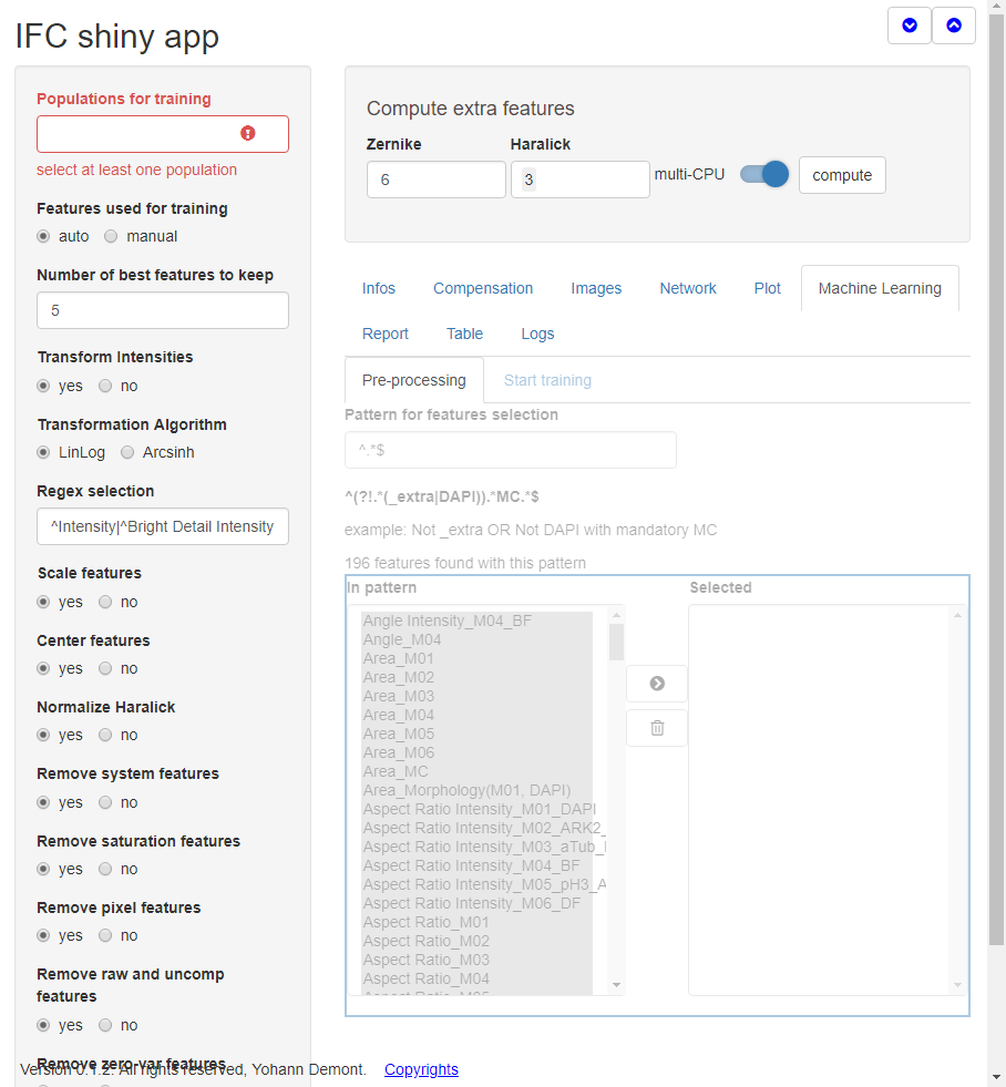
Once this is done almost everything can be done without much more user input by default. Nonetheless, the app allows for a lot of customization.

With Features used for training, you will be able to choose auto or manual. With manual you will be able to manually pick the features you wa