Option trading simulator

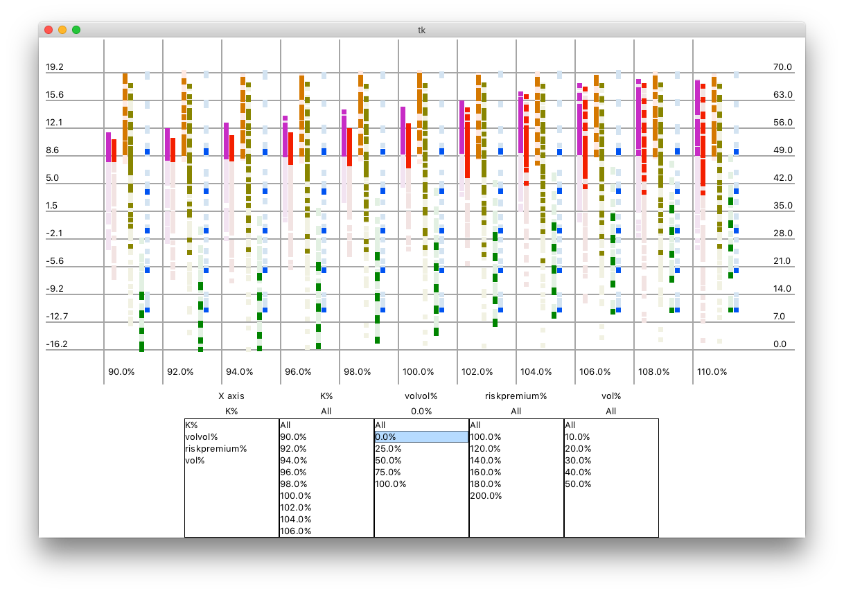
The first release contains only simulations for covered writes that are made exactly 30 days before expiration, and are always carried until the last day. This particular covered write strategy is useful to damp stock volatility and/or extract a steady income from a long-term stock position.

The three executable scripts are:

simulavc.py

Simulates a huge number of operations for a given scenario and prints the average return and volatility.

Note that calculated return and volatility are averages over many, many individual operations; they represent what a long-term investor would get upon doing the operation many times over an extended amount of time.

h_vc.py

Simulation supervisor: creates a list of scenarios based on market variables, and calls simulavc.py for each scenario, writing the result in a text file (data_vc.txt).

This script can be safely stopped, and scenario variables can even be changed. Scenarios already simulated (and written to text file) are skipped. Also, several simulations can be spawned in parallel (useful in multi-core computers: using two cores will cut the total simulation time by half).

g_vc.py

Simulation data graphic visualizer: for analysis of simulation results. Some filtering options are available, so the effect of each market variable can be pinpointed.

Graphics are plotted using Tk, which is the most portable option for Python. The downside is ugliness.

Scenario variables

Both in h_vc.py script and the graphic visualizer, the scenario variables can be seen, and we need to explain each one briefly.

K%: strike value as a percentage of spot. K=106% means that, for a stock with spot value of $100, strike would be $106 (that is, 6% out-of-the-money). For a stock with current value of $50, strike would be $53. And so on.

volvol%: "volatility of volatility". When this variable is bigger than zero, the distribution of returns is a leptokurtosis instead of normal. Unit is % of volatility. For example, if volatility is 30% and volvol is 50%, it means that standard deviation of volatility is 15%; the instantaneous volatility will fall between 15% and 45% twice in every three samples.

riskpremium%: The risk premium of the stock. For example, if interest rate is 9% and riskpremium is 150%, the instantaneous rate of return for the stock is 13.5%. (Note that volatility will depress this, so the actual rate of return would be lower.)

vol%: the volatility, expressed in %/year.

The interest rate is locked at 9% for all simulations.

Data format written to text file

In short, The data_vc.txt file has the following format:

• First line contains a list with all values of all market variables that have been/are to be combined in order to create scenarios. This line begins with '@'.

• All other lines contain simulation data. They begin with '#'.

For each simulation data line, the values mean:

• The first values, left to right, are the specific market variables for that scenario. The scenario generator uses them to determine which scenarios have already been simulated.

• Following them, we have the data actually generated by each simulation. In the case of covered writes, values are:

a) Average instantaneous rate of return of covered writes (always including the stock's own return, since the stock is part of the operation)

b) Average volatility of the covered write return;

c) Average rate of return of covered writes (which takes into account the fact that volatility reduces the rate of return).

d, e, f) Average return, volatility and corrected return for the raw stock. This is supplied to check the simulation and to be a basis of comparison against covered write.

Graphics format

Each scenario puts exactly six points in the graph, each one with a different color:

Purple: Instantaneous rate of return of stock position plus covered write

Red: Rate of return of stock position + covered write (smaller than instantaneous return because of volatility)

Dark Orange: Instantaneous rate of return of the stock position

Olive: Rate of return of the stock position

Dark Green: Volatility of the stock position + covered write.

Blue: Volatility of the stock position

The most interesting points are the Red and Green ones, since they tell the return rate and volatility for covered writes. The "raw" stock position returns and volatilities are plotted just for comparison and checking purposes.

X axis is the strike as a percentage of spot, but this can be changed; just select another variable at the leftmost ("X axis") list.

Y axis may be rate of return or volatility (depending on point color), both having %/year as unit. Left side shows scale for rate of return, right side shows scale for volatilty. Note that volatilities are always positive while rates of return may be negative.

At the bottom of graphics screen, the scenario variables are shown as lists. Clicking in a specific value puts the respective scenarios in evidence.

Fast Black-Scholes module and Psyco usage

There are a couple things you can do if you want/need the simulation to run faster. The cummulative gain is about 8x or more:

a) install Psyco.

b) compile the bsfast.pyx module, which reimplements selected Black-Scholes functions in Cython.