DNNHDL

Introduction

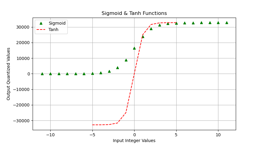
This project's initial goal is to simplify VHDL code generation for DNNs. It now covers techniques for hardware-efficient implementation of prevalent Activation Functions (AFs), i.e. Sigmoid and Tanh.

In the first section, which is based on LUT-based AFs, you will learn how to generate a .vhd file for those AFs by Python. The second section is more advanced and based on Piecewise-Linear (PWL) approximation technique.

Prerequisites

Python
Numpy
Matplotlib

1. LUT-based AFs

In this technique, nonlinear AFs are transformed into straight horizontal lines. This method is famous for its simplicity and computation. However, it lacks enough accuracy and normally its absolute error is higher than other methods with the same number of segments.

Steps

1. Clone the project in a folder and open it.
2. Set your values in the "Arbitrary inputs" section of the "sig_tanh_gen.py" file.
3. Run (in Windows):
   py .\sig_tanh_gen.py
   Or (in Linux):
   python sig_tanh_gen.py

With default inputs, you will see results similar to Fig. 1.

Also, you can see generated_sig.vhd and generated_tanh.vhd files in current folder.
You can play with arbitrary inputs and get your custom VHDL file.

2. PWL-based AFs

In this strategy, each segment of the main AF is transformed into straight lines and each straight line has its slope and y-intercept. This method is more resource-hungry than LUT-based and gives comparatively higher accuracy instead. POT_PWL.py is written scalable and you can change the input interval, number of segments, and input/output bit width. You can easily change the def sigmoid function and see the results.

This code gives you the slopes and y-intercepts of the straight lines that can be used to develop a .vhd file in FPGA. Simply, copy the values of slopes and y-intercepts to the c_slope and c_lat constants of the POT_PWL.vhd file, respectively.

Steps

Run POT_PWL.py similar to the steps of the previous section.

With default inputs, you will see results similar to Fig. 2 for the Sigmoid function. Notably, this Semi-sigmoid is similar to the original Sigmoid but shifted down by 1/2 for symmetry. Sigmoid Alpha and Beta are PWL approximations of the Sigmoid that are optimized for Mean Square Error (MSE) and Maximum Absolute Error (MXE), respectively.

You can also see the absolute error values like the following figure if you uncomment the corresponding line at the bottom of the code.

NB: If you find this project useful, I would appreciate your citing this repo. I would also be happy to hear any suggestions for improvement!