Data Structures and Algorithms in Java

Very useful in interview process for Java Software Development Engineer (SDE).

Big O Notation

Big-O Complexity Chart

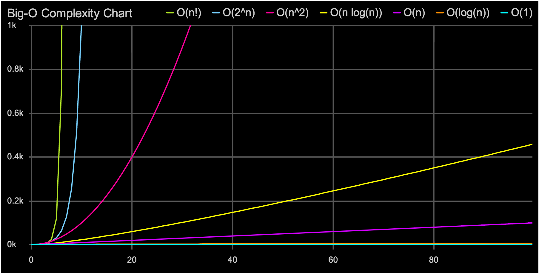
Constant — statement (one line of code)

a += 1;

Growth Rate: 1

Logarithmic — divide in half (binary search)

while (n > 1) {
  n = n / 2;
}

Growth Rate: log(n)

Linear — loop

for (int i = 0; i < n; i++) {
  // statements
  a += 1;
}

Growth Rate: n

The loop executes N times, so the sequence of statements also executes N times. If we assume the statements are O(1), the total time for the for loop is N * O(1), which is O(N) overall.

Quadratic — Effective sorting algorithms

Mergesort, Quicksort, …

Growth Rate: n*log(n)

Quadratic — double loop (nested loops)

for (int c = 0; c < n; c++) {
  for (int i = 0; i < n; i++) {
    // sequence of statements
    a += 1;
  }
}

Growth Rate: n^2

The outer loop executes N times. Every time the outer loop executes, the inner loop executes M times. As a result, the statements in the inner loop execute a total of N * M times. Thus, the complexity is O(N * M). In a common special case where the stopping condition of the inner loop is J < N instead of J < M (i.e., the inner loop also executes N times), the total complexity for the two loops is O(N2).

Cubic — triple loop

for (c = 0; c < n; c++) {
  for (i = 0; i < n; i++) {
    for (x = 0; x < n; x++) {
      a += 1;
    }
  }
}

Growth Rate: n^3

Exponential — exhaustive search

Trying to break a password generating all possible combinations

Growth Rate: 2^n

If-Then-Else

if (cond) {
  block 1 (sequence of statements)
} else {
  block 2 (sequence of statements)
}

If block 1 takes O(1) and block 2 takes O(N), the if-then-else statement would be O(N).

Statements with function/ procedure calls

When a statement involves a function/ procedure call, the complexity of the statement includes the complexity of the function/ procedure. Assume that you know that function/procedure f takes constant time, and that function/procedure g takes time proportional to (linear in) the value of its parameter k. Then the statements below have the time complexities indicated.

f(k) has O(1) g(k) has O(k)

When a loop is involved, the same rule applies. For example:

for J in 1 .. N loop
  g(J);
end loop;

has complexity (N2). The loop executes N times and each function/procedure call g(N) is complexity O(N).

Algorithms

Simple Sorting

Bubble Sort

Implementation

The bubble sort is notoriously slow, but it’s conceptually the simplest of the sorting algorithms.

Sorting process

1. Compare two items.
2. If the one on the left is bigger, swap them.
3. Move one position right.

Efficiency

For 10 data items, this is 45 comparisons (9 + 8 + 7 + 6 + 5 + 4 + 3 + 2 + 1).

In general, where N is the number of items in the array, there are N-1 comparisons on the first pass, N-2 on the second, and so on. The formula for the sum of such a series is (N–1) + (N–2) + (N–3) + ... + 1 = N*(N–1)/2 N*(N–1)/2 is 45 (10*9/2) when N is 10.

Selection Sort

Implementation

Simple explanation

The selection sort improves on the bubble sort by reducing the number of swaps necessary from O(N2) to O(N). Unfortunately, the number of comparisons remains O(N2). However, the selection sort can still offer a significant improvement for large records that must be physically moved around in memory, causing the swap time to be much more important than the comparison time.

Efficiency

The selection sort performs the same number of comparisons as the bubble sort: N*(N-1)/2. For 10 data items, this is 45 comparisons. However, 10 items require fewer than 10 swaps. With 100 items, 4,950 comparisons are required, but fewer than 100 swaps. For large values of N, the comparison times will dominate, so we would have to say that the selection sort runs in O(N2) time, just as the bubble sort did.

Insertion Sort

Implementation

Simple explanation

In most cases the insertion sort is the best of the elementary sorts described in this chapter. It still executes in O(N2) time, but it’s about twice as fast as the bubble sort and somewhat faster than the selection sort in normal situations. It’s also not too complex, although it’s slightly more involved than the bubble and selection sorts. It’s often used as the final stage of more sophisticated sorts, such as quicksort.

Efficiency

How many comparisons and copies does this algorithm require? On the first pass, it compares a maximum of one item. On the second pass, it’s a maximum of two items, and so on, up to a maximum of N-1 comparisons on the last pass. This is 1 + 2 + 3 + ... + N-1 = N*(N-1)/2

However, because on each pass an average of only half of the maximum number of items are actually compared before the insertion point is found, we can divide by 2, which gives N*(N-1)/4

The number of copies is approximately the same as the number of comparisons. However, a copy isn’t as time-consuming as a swap, so for random data this algorithm runs twice as fast as the bubble sort and faster than the selection sort.

In any case, like the other sort routines in this chapter, the insertion sort runs in O(N2) time for random data.

For data that is already sorted or almost sorted, the insertion sort does much better. When data is in order, the condition in the while loop is never true, so it becomes a simple statement in the outer loop, which executes N-1 times. In this case the algorithm runs in O(N) time. If the data is almost sorted, insertion sort runs in almost O(N) time, which makes it a simple and efficient way to order a file that is only slightly out of order.

Advanced Sorting

Merge Sort

Implementation

Simple explanation

mergesort is a much more efficient sorting technique than those we saw in "Simple Sorting", at least in terms of speed. While the bubble, insertion, and selection sorts take O(N2) time, the mergesort is O(N*logN).

For example, if N (the number of items to be sorted) is 10,000, then N2 is 100,000,000, while N*logN is only 40,000. If sorting this many items required 40 seconds with the mergesort, it would take almost 28 hours for the insertion sort.

The mergesort is also fairly easy to implement. It’s conceptually easier than quicksort and the Shell short.

The heart of the mergesort algorithm is the merging of two already-sorted arrays. Merging two sorted arrays A and B creates a third array, C, that contains all the elements of A and B, also arranged in sorted order.

Similar to quicksort the list of element which should be sorted is divided into two lists. These lists are sorted independently and then combined. During the combination of the lists the elements are inserted (or merged) on the correct place in the list.

You divide the half into two quarters, sort each of the quarters, and merge them to make a sorted half.

Sorting process

1. Assume the size of the left array is k, the size of the right array is m and the size of the total array is n (=k+m).
2. Create a helper array with the size n
3. Copy the elements of the left array into the left part of the helper array. This is position 0 until k-1.
4. Copy the elements of the right array into the right part of the helper array. This is position k until m-1.
5. Create an index variable i=0; and j=k+1
6. Loop over the left and the right part of the array and copy always the smallest value back into the original array. Once i=k all values have been copied back the original array. The values of the right array are already in place.

Efficiency

As we noted, the mergesort runs in O(N*logN) time. There are 24 copies necessary to sort 8 items. Log28 is 3, so 8*log28 equals 24. This shows that, for the case of 8 items, the number of copies is proportional to N*log2N.

In the mergesort algorithm, the number of comparisons is always somewhat less than the number of copies.

Comparison with Quicksort

Compared to quicksort the mergesort algorithm puts less effort in dividing the list but more into the merging of the solution.

Quicksort can sort "inline" of an existing collection, e.g. it does not have to create a copy of the collection while Standard mergesort does require a copy of the array although there are (complex) implementations of mergesort which allow to avoid this copying.

Quick Sort

![Quick Sort animation](https:/