TightBinding.jl

This can construct the tight-binding model and calculate energies in Julia 1.0. This software is released under the MIT License, see LICENSE. We checked that it works in Julia 1.7.

This can

1. construct the Hamiltonian as a functional of a momentum k.
2. plot the band structure.
3. show the crystal structure.
4. plot the band structure of the finite-width system with one surface or boundary.
5. [09 Feb. 2019] make surface Hamiltonian from the momentum space Hamiltonian.
6. [19 Nov. 2019] get DOS data and energy mesh
7. [22 Jun. 2020] construct a supercell model
8. [EXPERIMENTAL][22 Jun. 2020] write Wannier90 format.

There is the sample jupyter notebook.

Install

Push "]" to enter the package mode.

add TightBinding

samples

Graphene

Here is a Graphene case

using TightBinding
#Primitive vectors
a1 = [sqrt(3)/2,1/2]
a2= [0,1]
#set lattice
la = set_Lattice(2,[a1,a2])
#add atoms
add_atoms!(la,[1/3,1/3])
add_atoms!(la,[2/3,2/3])

Then we added two atoms (atom 1 and atom 2). We can see the possible hoppings.

show_neighbors(la)

Output is

Possible hoppings
(1,1), x:-1//1, y:-1//1
(1,2), x:-2//3, y:-2//3
(2,2), x:-1//1, y:-1//1
(1,1), x:-1//1, y:0//1
(1,2), x:-2//3, y:1//3
(2,2), x:-1//1, y:0//1
(1,1), x:-1//1, y:1//1
(1,2), x:-2//3, y:4//3
(2,2), x:-1//1, y:1//1
(1,1), x:0//1, y:-1//1
(1,2), x:1//3, y:-2//3
(2,2), x:0//1, y:-1//1
(1,1), x:0//1, y:0//1
(1,2), x:1//3, y:1//3
(2,2), x:0//1, y:0//1
(1,1), x:0//1, y:1//1
(1,2), x:1//3, y:4//3
(2,2), x:0//1, y:1//1
(1,1), x:1//1, y:-1//1
(1,2), x:4//3, y:-2//3
(2,2), x:1//1, y:-1//1
(1,1), x:1//1, y:0//1
(1,2), x:4//3, y:1//3
(2,2), x:1//1, y:0//1
(1,1), x:1//1, y:1//1
(2,2), x:1//1, y:1//1

If you want to construct the Graphene, you choose hoppings from atom 1 to atom 2:

#construct hoppings
t = 1.0
add_hoppings!(la,-t,1,2,[1/3,1/3])
add_hoppings!(la,-t,1,2,[-2/3,1/3])
add_hoppings!(la,-t,1,2,[1/3,-2/3])

using Plots
#show the lattice structure
plot_lattice_2d(la)

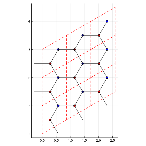
using Plots
# Density of states
nk = 100 #numer ob meshes. nk^d meshes are used. d is a dimension.
plot_DOS(la, nk)

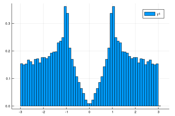
[19 Nov. 2019] We can get DOS data and energy mesh.

nk = 100 #numer ob meshes. nk^d meshes are used. d is a dimension.
hist = get_DOS(la, nk)
println(hist.weights) #DOS data
println(hist.edges[1]) #energy mesh
using Plots
plot(hist.edges[1][2:end] .- hist.edges[1].step.hi/2,hist.weights)

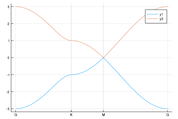
#show the band structure
klines = set_Klines()
kmin = [0,0]
kmax = [2π/sqrt(3),0]
add_Kpoints!(klines,kmin,kmax,"G","K")

kmin = [2π/sqrt(3),0]
kmax = [2π/sqrt(3),2π/3]
add_Kpoints!(klines,kmin,kmax,"K","M")

kmin = [2π/sqrt(3),2π/3]
kmax = [0,0]
add_Kpoints!(klines,kmin,kmax,"M","G")
calc_band_plot(klines,la)

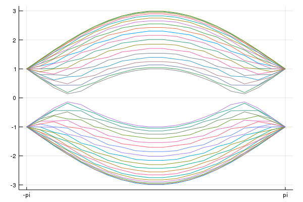
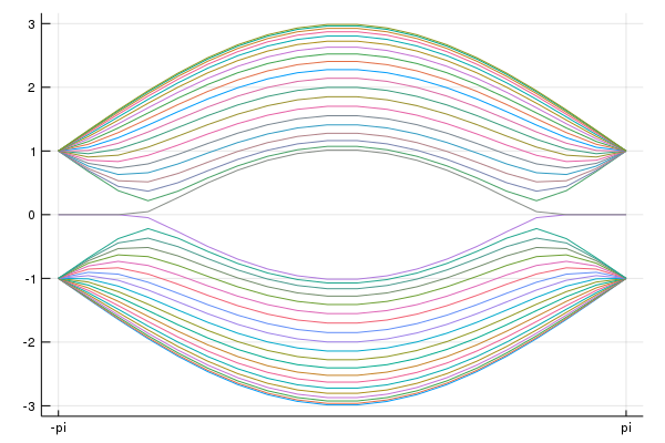
Graphene nano-ribbon

using Plots
#We have already constructed atoms and hoppings.
#We add the line to plot
klines = set_Klines()
kmin = [-π]
kmax = [π]
add_Kpoints!(klines,kmin,kmax,"-pi","pi")

#We consider the periodic boundary condition along the primitive vector
direction = 1
#Periodic boundary condition
calc_band_plot_finite(klines,la,direction,periodic=true)

#We introduce the surface perpendicular to the premitive vector
direction = 1
#Open boundary condition
calc_band_plot_finite(klines,la,direction,periodic=false)

Fe-based superconductor

We construct two-band model for Fe-based superconductor [S. Rachu et al. Phys. Rev. B 77, 220503(R) (2008)].

la = set_Lattice(2,[[1,0],[0,1]]) #Square lattice
add_atoms!(la,[0,0]) #dxz orbital
add_atoms!(la,[0,0]) #dyz orbital
#hoppings
t1 = -1.0
t2 = 1.3
t3 = -0.85
t4 = t3
μ = 1.45

#dxz
add_hoppings!(la,-t1,1,1,[1,0])
add_hoppings!(la,-t2,1,1,[0,1])
add_hoppings!(la,-t3,1,1,[1,1])
add_hoppings!(la,-t3,1,1,[1,-1])

#dyz
add_hoppings!(la,-t2,2,2,[1,0])
add_hoppings!(la,-t1,2,2,[0,1])
add_hoppings!(la,-t3,2,2,[1,1])
add_hoppings!(la,-t3,2,2,[1,-1])

#between dxz and dyz
add_hoppings!(la,-t4,1,2,[1,1])
add_hoppings!(la,-t4,1,2,[-1,-1])
add_hoppings!(la,t4,1,2,[1,-1])
add_hoppings!(la,t4,1,2,[-1,1])

#Chemical potentials
set_μ!(la,μ) #set the chemical potential

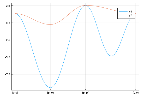
To see the band structure, we use

klines = set_Klines()
kmin = [0,0]
kmax = [π,0]
add_Kpoints!(klines,kmin,kmax,"(0,0)","(pi,0)")

kmin = [π,0]
kmax = [π,π]
add_Kpoints!(klines,kmin,kmax,"(pi,0)","(pi,pi)")

kmin = [π,π]
kmax = [0,0]
add_Kpoints!(klines,kmin,kmax,"(pi,pi)","(0,0)")

using Plots
pls = calc_band_plot(klines,la)

Then, we have the band structure:

We can obtain the Hamiltonian:

ham = hamiltonian_k(la) #we can obtain the function "ham([kx,ky])".
kx = 0.1
ky = 0.2
hamk = ham([kx,ky]) #ham is a functional of k=[kx,ky].
println(hamk)

Fe-based superconductor: 5 orbital model

Finally, we show the 5-orbital model proposed by K. Kuroki et al.[K. Kuroki et al., Phys. Rev. Lett. 101, 087004 (2008)]. The sample code is

la = set_Lattice(2,[[1,0],[0,1]])
add_atoms!(la,[0,0])
add_atoms!(la,[0,0])
add_atoms!(la,[0,0])
add_atoms!(la,[0,0])
add_atoms!(la,[0,0])

tmat = [
-0.7    0 -0.4  0.2 -0.1
-0.8    0    0    0    0
 0.8 -1.5    0    0 -0.3
   0  1.7    0    0 -0.1
-3.0    0    0 -0.2    0
-2.1  1.5    0    0    0
 1.3    0  0.2 -0.2    0
 1.7    0    0  0.2    0
-2.5  1.4    0    0    0
-2.1  3.3    0 -0.3  0.7
 1.7  0.2    0  0.2    0
 2.5    0    0  0.3    0
 1.6  1.2 -0.3 -0.3 -0.3
   0    0    0 -0.1    0
 3.1 -0.7 -0.2    0    0
]
tmat = 0.1.*tmat
imap = zeros(Int64,5,5)
count = 0
for μ=1:5
    for ν=μ:5
        count += 1
        imap[μ,ν] = count
    end
end
Is = [1,-1,-1,1,1,1,1,-1,-1,1,-1,-1,1,1,1]
σds = [1,-1,1,1,-1,1,-1,-1,1,1,1,-1,1,-1,1]
tmat_σy = tmat[:,:]
tmat_σy[imap[1,2],:] = -tmat[imap[1,3],:]
tmat_σy[imap[1,3],:] = -tmat[imap[1,2],:]
tmat_σy[imap[1,4],:] = -tmat[imap[1,4],:]
tmat_σy[imap[2,2],:] = tmat[imap[3,3],:]
tmat_σy[imap[2,4],:] = tmat[imap[3,4],:]
tmat_σy[imap[2,5],:] = -tmat[imap[3,5],:]
tmat_σy[imap[3,3],:] = tmat[imap[2,2],:]
tmat_σy[imap[3,4],:] = tmat[imap[2,4],:]
tmat_σy[imap[3,5],:] = -tmat[imap[2,5],:]
tmat_σy[imap[4,5],:] = -tmat[imap[4,5],:]

hoppingmatrix = zeros(Float64,5,5,5,5)
hops = [-2,-1,0,1,2]
hopelements = [[1,0],[1,1],[2,0],[2,1],[2,2]]

for μ = 1:5
    for ν=μ:5
        for ii=1:5
            ihop = hopelements[ii][1]
            jhop = hopelements[ii][2]
            #[a,b],[a,-b],[-a,-b],[-a,b],[b,a],[b,-a],[-b,a],[-b,-a]

            #[a,b]
            i = ihop +3
            j = jhop +3
            hoppingmatrix[μ,ν,i,j]=tmat[imap[μ,ν],ii]
            #[a,-b] = σy*[a,b] [1,1] -> [1,-1]
            if jhop != 0
                i = ihop +3
                j = -jhop +3
                hoppingmatrix[μ,ν,i,j]=tmat_σy[imap[μ,ν],ii]
            end

            if μ != ν
                #[-a,-b] = I*[a,b] [1,1] -> [-1,-1],[1,0]->[-1,0]
                i = -ihop +3
                j = -jhop +3
                hoppingmatrix[μ,ν,i,j]=Is[imap[μ,ν]]*tmat[imap[μ,ν],ii]
                #[-a,b] = I*[a,-b] = I*σy*[a,b]  #[2,0]->[-2,0]
                if jhop != 0
                    i = -ihop +3
                    j = jhop +3
                    hoppingmatrix[μ,ν,i,j]=Is[imap[μ,ν]]*tmat_σy[imap[μ,ν],ii]
                end
            end
            #[b,a],[b,-a],[-b,a],[-b,-a]
            if jhop != ihop
                #[b,a] = σd*[a,b]
                i = jhop +3
                j = ihop +3
                hoppingmatrix[μ,ν,i,j]=σds[imap[μ,ν]]*tmat[imap[μ,ν],ii]
                #[-b,a] = σd*σy*[a,b]
                if jhop != 0
                    i = -jhop +3
                    j = ihop +3
                    hoppingmatrix[μ,ν,i,j]=σds[imap[μ,ν]]*tmat_σy[imap[μ,ν],ii]
                end

                if μ != ν
                    #[-b,-a] = σd*[-a,-b] = σd*I*[a,b]
                    i = -jhop +3
                    j = -ihop +3
                    hoppingmatrix[μ,ν,i,j]=σds[imap[μ,ν]]*Is[imap[μ,ν]]*tmat[imap[μ,ν],ii]
                    #[b,-a] = σd*[-a,b] = σd*I*[a,-b] = σd*I*σy*[a,b]  #[2,0]->[-2,0]
                    if jhop != 0
                        i = jhop +3