diffeqpy

diffeqpy is a package for solving differential equations in Python. It utilizes DifferentialEquations.jl for its core routines to give high performance solving of many different types of differential equations, including:

• Discrete equations (function maps, discrete stochastic (Gillespie/Markov) simulations)
• Ordinary differential equations (ODEs)
• Split and Partitioned ODEs (Symplectic integrators, IMEX Methods)
• Stochastic ordinary differential equations (SODEs or SDEs)
• Random differential equations (RODEs or RDEs)
• Differential algebraic equations (DAEs)
• Delay differential equations (DDEs)
• Mixed discrete and continuous equations (Hybrid Equations, Jump Diffusions)

directly in Python.

If you have any questions, or just want to chat about solvers/using the package, please feel free to chat in the Gitter channel. For bug reports, feature requests, etc., please submit an issue.

Installation

To install diffeqpy, use pip:

pip install diffeqpy

and you're good!

Colab Notebook Examples

• Solving the Lorenz equation faster than SciPy+Numba
• Solving ODEs on GPUs Fast in Python with diffeqpy

General Flow

Import and setup the solvers available in DifferentialEquations.jl via the command:

from diffeqpy import de

If only the solvers available in OrdinaryDiffEq.jl are required, then use the command:

from diffeqpy import ode

The general flow for using the package is to follow exactly as would be done in Julia, except add de. or ode. in front. Note that ode. has a shorter loading time and a smaller memory footprint compared to de.. Most of the commands will work without any modification. Thus the DifferentialEquations.jl documentation and the DiffEqTutorials are the main in-depth documentation for this package. Below we will show how to translate these docs to Python code.

Note about !

Python does not allow ! in function names, so this is also a limitation of pyjulia. To use functions which on the Julia side have a !, like step!, replace ! by _b. For example:

from diffeqpy import de

def f(u,p,t):
    return -u

u0 = 0.5
tspan = (0., 1.)
prob = de.ODEProblem(f, u0, tspan)
integrator = de.init(prob, de.Tsit5())
de.step_b(integrator)

is valid Python code for using the integrator interface.

Ordinary Differential Equation (ODE) Examples

One-dimensional ODEs

from diffeqpy import de

def f(u,p,t):
    return -u

u0 = 0.5
tspan = (0., 1.)
prob = de.ODEProblem(f, u0, tspan)
sol = de.solve(prob)

The solution object is the same as the one described in the DiffEq tutorials and in the solution handling documentation (note: the array interface is missing). Thus for example the solution time points are saved in sol.t and the solution values are saved in sol.u. Additionally, the interpolation sol(t) gives a continuous solution.

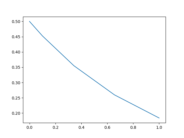
We can plot the solution values using matplotlib:

import matplotlib.pyplot as plt
plt.plot(sol.t,sol.u)
plt.show()

We can utilize the interpolation to get a finer solution:

import numpy
t = numpy.linspace(0,1,100)
u = sol(t)
plt.plot(t,u)
plt.show()

Solve commands

The common interface arguments can be used to control the solve command. For example, let's use saveat to save the solution at every t=0.1, and let's utilize the Vern9() 9th order Runge-Kutta method along with low tolerances abstol=reltol=1e-10:

sol = de.solve(prob,de.Vern9(),saveat=0.1,abstol=1e-10,reltol=1e-10)

The set of algorithms for ODEs is described at the ODE solvers page.

Compilation with de.jit and Julia

When solving a differential equation, it's pertinent that your derivative function f is fast since it occurs in the inner loop of the solver. We can convert the entire ode problem to symbolic form, optimize that symbolic form, and emit efficient native code to simulate it using de.jit to improve the efficiency of the solver at the expense of added setup time:

fast_prob = de.jit(prob)
sol = de.solve(fast_prob)

Additionally, you can directly define the functions in Julia. This will also allow for specialization and could be helpful to increase the efficiency for repeat or long calls. This is done via seval:

jul_f = de.seval("(u,p,t)->-u") # Define the anonymous function in Julia
prob = de.ODEProblem(jul_f, u0, tspan)
sol = de.solve(prob)

Limitations

de.jit, uses ModelingToolkit.jl's modelingtoolkitize internally and some restrictions apply. Not all models can be jitted. See the modelingtoolkitize documentation for more info.

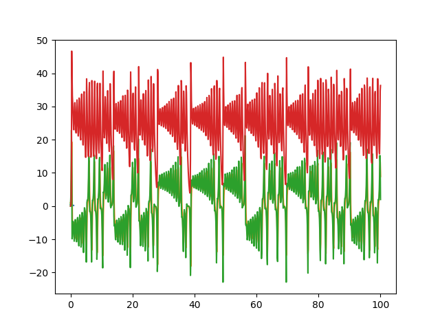
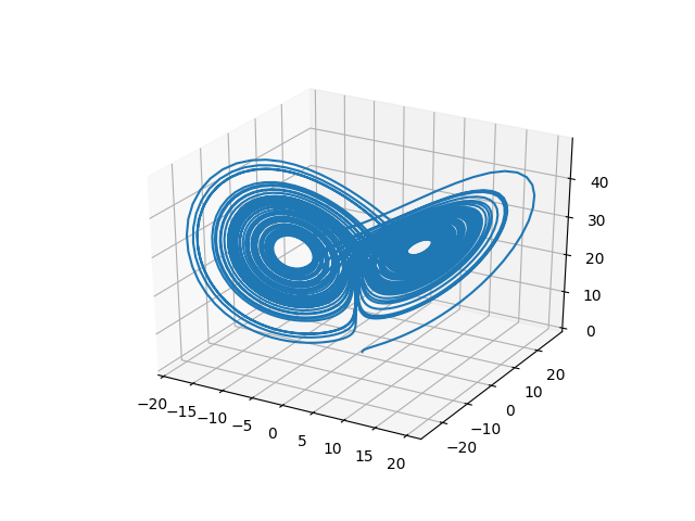
Systems of ODEs: Lorenz Equations

To solve systems of ODEs, simply use an array as your initial condition and define f as an array function:

def f(u,p,t):
    x, y, z = u
    sigma, rho, beta = p
    return [sigma * (y - x), x * (rho - z) - y, x * y - beta * z]

u0 = [1.0,0.0,0.0]
tspan = (0., 100.)
p = [10.0,28.0,8/3]
prob = de.ODEProblem(f, u0, tspan, p)
sol = de.solve(prob,saveat=0.01)

plt.plot(sol.t,de.transpose(de.stack(sol.u)))
plt.show()

or we can draw the phase plot:

us = de.stack(sol.u)
from mpl_toolkits.mplot3d import Axes3D
fig = plt.figure()
ax = fig.add_subplot(111, projection='3d')
ax.plot(us[0,:],us[1,:],us[2,:])
plt.show()

In-Place Mutating Form

When dealing with systems of equations, in many cases it's helpful to reduce memory allocations by using mutating functions. In diffeqpy, the mutating form adds the mutating vector to the front. Let's make a fast version of the Lorenz derivative, i.e. mutating and JIT compiled:

def f(du,u,p,t):
    x, y, z = u
    sigma, rho, beta = p
    du[0] = sigma * (y - x)
    du[1] = x * (rho - z) - y
    du[2] = x * y - beta * z

u0 = [1.0,0.0,0.0]
tspan = (0., 100.)
p = [10.0,28.0,2.66]
prob = de.ODEProblem(f, u0, tspan, p)
jit_prob = de.jit(prob)
sol = de.solve(jit_prob)

or using a Julia function:

jul_f = de.seval("""
function f(du,u,p,t)
  x, y, z = u
  sigma, rho, beta = p
  du[1] = sigma * (y - x)
  du[2] = x * (rho - z) - y
  du[3] = x * y - beta * z
end""")
u0 = [1.0,0.0,0.0]
tspan = (0., 100.)
p = [10.0,28.0,2.66]
prob = de.ODEProblem(jul_f, u0, tspan, p)
sol = de.solve(prob)

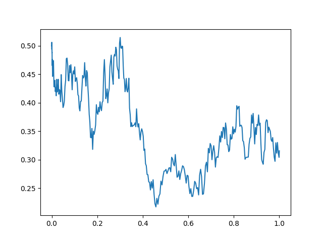
Stochastic Differential Equation (SDE) Examples

One-dimensional SDEs

Solving one-dimensonal SDEs du = f(u,t)dt + g(u,t)dW_t is like an ODE except with an extra function for the diffusion (randomness or noise) term. The steps follow the SDE tutorial.

def f(u,p,t):
  return 1.01*u

def g(u,p,t):
  return 0.87*u

u0 = 0.5
tspan = (0.0,1.0)
prob = de.SDEProblem(f,g,u0,tspan)
sol = de.solve(prob,reltol=1e-3,abstol=1e-3)

plt.plot(sol.t,de.stack(sol.u))
plt.show()

Systems of SDEs with Diagonal Noise

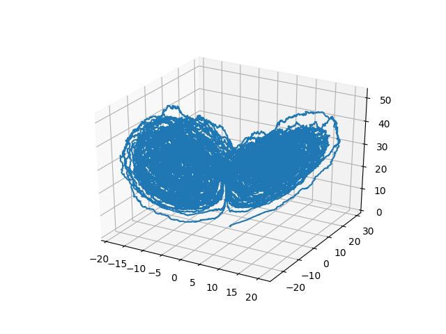
An SDE with diagonal noise is where a different Wiener process is applied to every part of the system. This is common for models with phenomenological noise. Let's add multiplicative noise to the Lorenz equation:

def f(du,u,p,t):
    x, y, z = u
    sigma, rho, beta = p
    du[0] = sigma * (y - x)
    du[1] = x * (rho - z) - y
    du[2] = x * y - beta * z

def g(du,u,p,t):
    du[0] = 0.3*u[0]
    du[1] = 0.3*u[1]
    du[2] = 0.3*u[2]

u0 = [1.0,0.0,0.0]
tspan = (0., 100.)
p = [10.0,28.0,2.66]
prob = de.jit(de.SDEProblem(f, g, u0, tspan, p))
sol = de.solve(prob)

# Now let's draw a phase plot

us = de.stack(sol.u)
from mpl_toolkits.mplot3d import Axes3D
fig = plt.figure()
ax = fig.add_subplot(111, projection='3d')
ax.plot(us[0,:],us[1,:],us[2,:])
plt.show()

Systems of SDEs with Non-Diagonal Noise

In many cases you may want to share noise terms across the system. This is known as non-diagonal noise. The DifferentialEquations.jl SDE Tutorial explains how the matrix form of the diffusion term corresponds to the summation style of multiple Wiener processes. Essentia