DPFEHM: A Differentiable Subsurface Physics Simulator

Description

DPFEHM is a Julia module that includes differentiable numerical models with a focus on the Earth's subsurface, especially fluid flow. Currently it supports the groundwater flow equations (single phase flow), Richards equation (air/water), the advection-dispersion equation, and the 2d wave equation. Since it is differentiable, it can easily be combined with machine learning models in a workflow such as this:

This workflow shows how to train a machine learning model to mitigate problems with injecting fluid into the earth's subsurface (such as induced seismicity or leakage of carbon dioxide). More details on this workflow are available here.

Installation

Within Julia, you can install DPFEHM and test that it works by running

import Pkg
Pkg.add("DPFEHM")
Pkg.test("DPFEHM")

Basic Usage

The examples are a good place to get started to see how to use DPFEHM. Two examples will be described in detail here that illustrate the basic usage patterns via an examples of steady-state single-phase flow and transient Richards equation.

Steady-state single-phase flow

Here, we solve a steady-state single phase flow problem . Let's start by importing several libraries that we will use.

import DPFEHM
import GaussianRandomFields
import Optim
import PyPlot
import Random
import Zygote
Random.seed!(0)#set the seed so we can reproduce the same results with each run

Next, we'll set up the grid. Here, we use a regular grid with 100,000 nodes that covers a domain that is 50 meters by 50 meters by 5 meters.

mins = [0, 0, 0]; maxs = [50, 50, 5]#size of the domain, in meters
ns = [100, 100, 10]#number of nodes on the grid
coords, neighbors, areasoverlengths, _ = DPFEHM.regulargrid3d(mins, maxs, ns)#build the grid

The result of this grid-building is three variables that we will use. The, coords is a matrix describing the coordinates of the cell centers on the grid. The second, neighbors, is an array describing which cells neighbor other cells. The third, areasoverlengths, is another array whose length is equal to the length of neighbors and describes the area of the interface between two neighboring cells dividing by the length between the cell centers. The last variable is dumped to _ and gives the volumes of the cells. The volumes of the cells are not needed for steady state problems, so they are not used in this example.

Now we set up the boundary conditions.

Qs = zeros(size(coords, 2))
injectionnode = 1#inject in the lower left corner
Qs[injectionnode] = 1e-4#m^3/s
dirichletnodes = Int[size(coords, 2)]#fix the pressure in the upper right corner
dirichleths = zeros(size(coords, 2))
dirichleths[size(coords, 2)] = 0.0

The variable Qs describes fluid sources/sinks -- the amount of fluid injected at cell i on the grid is given by Qs[i]. In this example, the only place were we inject fluid is at node 1. Another variable, dirichletnodes is a list of cells at which the pressure will be fixed. In this example, the pressure is fixed at the last cell, which is cell number size(coords, 2). The variable dirichleths describes the pressures (or heads in hydrology jargon) that the cells are fixed at. Note that the length of dirichleths is size(coords, 2), but these values are ignored except at the indices that appear in dirichletnodes.

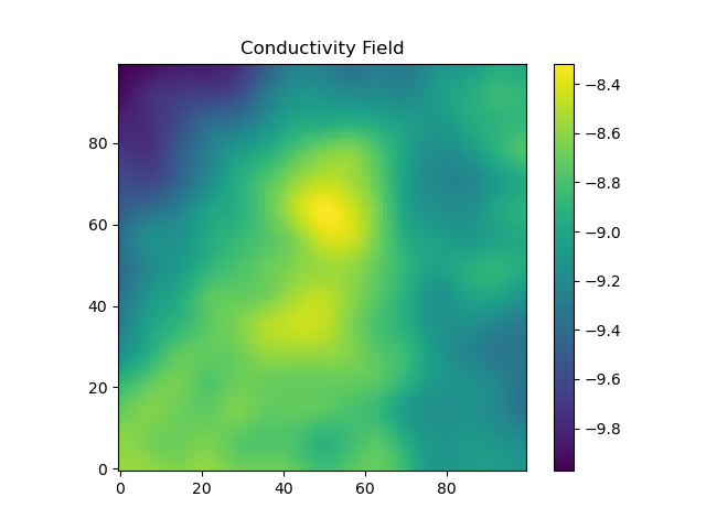
The final set-up step before moving on to solving the equations is to construct a heterogeneous conductivity field. Here, we use the package GaussianRandomFields to construct a conductivity field with a correlation length of 50 meters. The mean of the log-conductivity is 1e-4meters/second (note that we use a natural logarithm when defining this), and the standard deviation of the log-conductivity is 1. GaussianRandomFields is used to construct a field in 2 dimensions and then it is copied through each of the layers, so that the heterogeneity only exists in the x and y coordinate directions, but not in the z direction.

lambda = 50.0#meters -- correlation length of log-conductivity
sigma = 1.0#standard deviation of log-conductivity
mu = -9.0#mean of log conductivity -- ~1e-4 m/s, like clean sand here https://en.wikipedia.org/wiki/Hydraulic_conductivity#/media/File:Groundwater_Freeze_and_Cherry_1979_Table_2-2.png
cov = GaussianRandomFields.CovarianceFunction(2, GaussianRandomFields.Matern(lambda, 1; σ=sigma))
x_pts = range(mins[1], maxs[1]; length=ns[1])
y_pts = range(mins[2], maxs[2]; length=ns[2])
num_eigenvectors = 200
grf = GaussianRandomFields.GaussianRandomField(cov, GaussianRandomFields.KarhunenLoeve(num_eigenvectors), x_pts, y_pts)
logKs = zeros(reverse(ns)...)
logKs2d = mu .+ GaussianRandomFields.sample(grf)'#generate a random realization of the log-conductivity field
for i = 1:ns[3]#copy the 2d field to each of the 3d layers
	v = view(logKs, i, :, :)
	v .= logKs2d
end

The conductivity field is shown:

<!-- #plot the log-conductivity fig, ax = PyPlot.subplots() img = ax.imshow(logKs[1, :, :], origin="lower") ax.title.set_text("Conductivity Field") fig.colorbar(img) display(fig) println() PyPlot.close(fig) -->

Now, we look to solve the flow problem. First, we define a helper function, logKs2Ks_neighbors. This function is needed because the flow solver wants to know the conductivity on the interface between two cells, but our previous construction defined the conductivities at the cells themselves. It also converts from log-conductivity to conductivity and uses the geometric mean to move from the cells to the interfaces. The heart of this code is the call to DPFEHM.groundwater_steadystate, which solves the single phase steady-state flow problem that we pose. The solveforh function calls this function and returns the result after reshaping.

logKs2Ks_neighbors(Ks) = exp.(0.5 * (Ks[map(p->p[1], neighbors)] .+ Ks[map(p->p[2], neighbors)]))#convert from permeabilities at the nodes to permeabilities connecting the nodes
function solveforh(logKs, dirichleths)
	@assert length(logKs) == length(Qs)
	Ks_neighbors = logKs2Ks_neighbors(logKs)
	return reshape(DPFEHM.groundwater_steadystate(Ks_neighbors, neighbors, areasoverlengths, dirichletnodes, dirichleths, Qs), reverse(ns)...)
	end
end

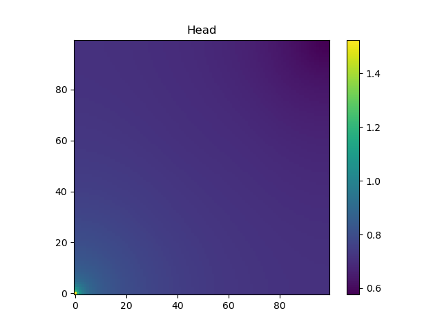
With this function in hand, we can solve the problem using the solveforh wrapper function we previously defined. This function requires us to explicitly pass in logKs (the hydraulic conductivity) and dirichleths (the fixed-head boundary condition), but the other inputs to DPFEHM.groundwater_steadystate are fixed to global values.

h = solveforh(logKs, dirichleths)#solve for the head

The head at the bottom layer of the domain is shown (note the pressure is higher in the lower corner, where there is fluid injection, than in the rest of the domain):

<!-- #plot the head at the bottom of the domain fig, ax = PyPlot.subplots() img = ax.imshow(h[1, :, :], origin="lower") ax.title.set_text("Head") fig.colorbar(img) display(fig) println() PyPlot.close(fig) -->

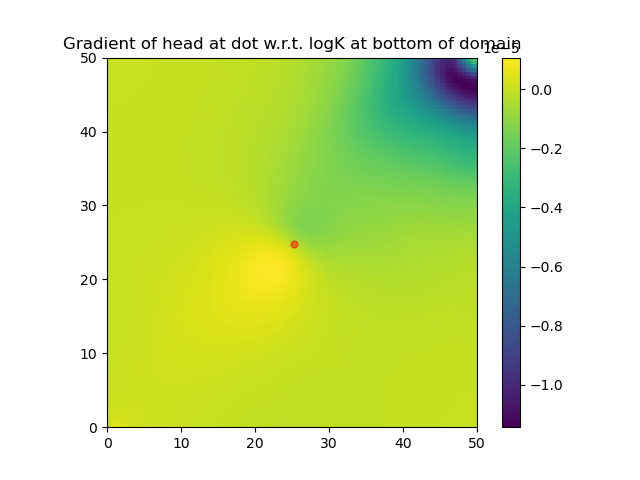
DPFEHM also allows us to compute the gradient of functions involving DPFEHM.groundwater_steadystate using Zygote.gradient or Zygote.pullback.

isfreenode, nodei2freenodei, freenodei2nodei = DPFEHM.getfreenodes(length(dirichleths), dirichletnodes)
gradient_node = nodei2freenodei[div(size(coords, 2), 2) + 500]
gradient_node_x = coords[1, gradient_node]
gradient_node_y = coords[2, gradient_node]
grad = Zygote.gradient((x, y)->solveforh(x, y)[gradient_node], logKs, dirichleths)#calculate the gradient (which involves a redundant calculation of the forward pass)
function_evaluation, back = Zygote.pullback((x, y)->solveforh(x, y)[gradient_node], logKs, dirichleths)#this pullback thing lets us not redo the forward pass
print("gradient time")
grad2 = back(1.0)#compute the gradient of a function involving solveforh using Zygote.pullback

Note that the function DPFEHM.getfreenodes allows one to map indices between the free nodes (i.e., the ones that do not have fixed-pressure boundary conditions) and all nodes. The gradient of logK at the bottom layer of the domain is shown:

<!-- #plot the gradient of the function w.r.t. the logK at the bottom of the domain fig, ax = PyPlot.subplots() img = ax.imshow(grad[1][1, :, :], origin="lower", extent=[mins[1], maxs[1], mins[2], maxs[2]]) ax.plot([gradient_node_x], [gradient_node_y], "r.", ms=10, alpha=0.5) ax.title.set_text("Gradient of head at dot w.r.t. logK at bottom of domain") fig.colorbar(img) display(fig) println() PyPlot.close(fig) -->

Transient Richards flow

Now, we consider an example using DPFEHM's solver for Richards equation, which can be used to model flow in a porous medium where both air and water fill the pores (i.e., unsaturated flow). This example is similar to the previous example and we again start by importing several li