OTSOpy

Python package version of the OTSO tool used for trajectory computations of charged particles in the Earth's magnetosphere.

OTSO is designed to be open-source; all suggestions for improvement are welcome, and please report any bugs you find. I welcome any help provided by the community in the development of OTSO.

Supported Python Versions: 3.10, 3.11, 3.12, 3.13, and 3.14 (I will endeavour to keep OTSO support as up to date as possible)

OTSO Documentation

Detailed OTSO documentation for functions and input parameters is provided digitally via GitHub pages. Documentation can be found by clicking on OTSOdocs.

Installation

Installation of OTSOpy is designed to be as simple as possible and can be done utilising pip. Users have two options when downloading OTSOpy.

Option 1: PyPi

Users may install OTSO directly from PyPi using:

pip install OTSO

This will install OTSO into your current Python environment.

Option 2: Repository

Users may clone the repository and run the setup.py file within the main OTSOpy directory using:

pip install .

This will install OTSO into your current Python environment.

Troubleshooting

LINUX

Sometimes there are errors regarding libgfortran. Make a note of the libgfortran error message and then install the appropriate libgfortran version that is being requested. This should resolve the issue.

MAC

The compiled fortran libraries can be flagged as potential malware. To resolve this you can attempt to compile the libraries yourself or in your settings grant permission for your computer to access the required .so file.

Functions

Cutoff

Computes the geomagnetic cut-off rigidities for given locations around the Earth under user-inputted geomagnetic conditions.

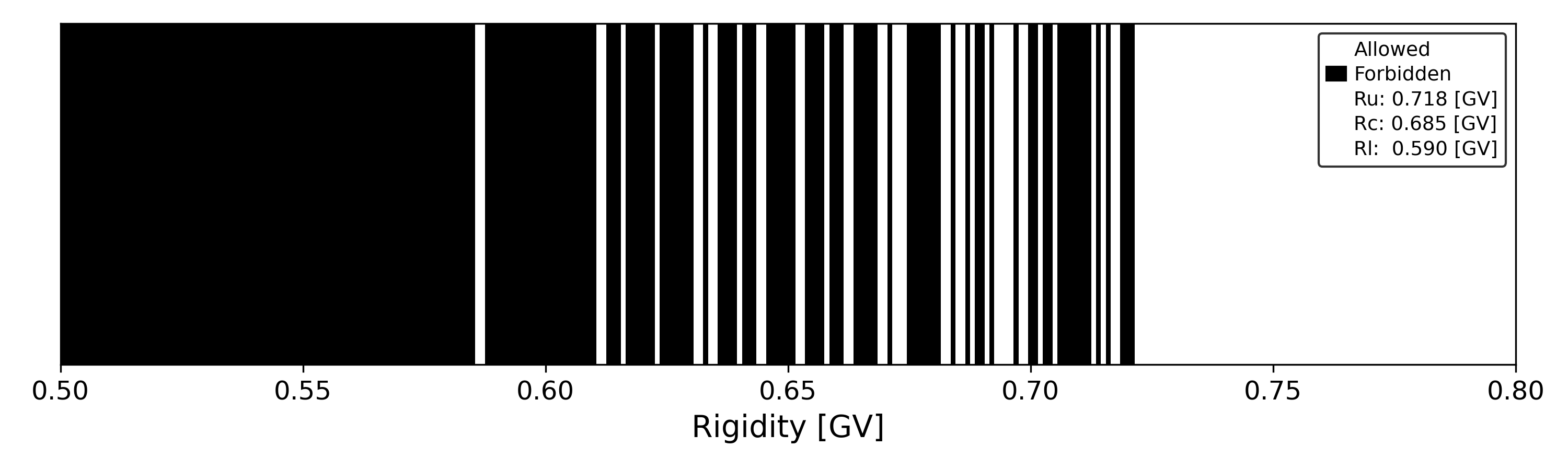Figure 1: Computation of the Oulu neutron monitor effective cut-off rigidity using the IGRF 2000 epoch and TSY89 model with kp index = 0. Penumbra is shown by the forbidden and allowed trajectories being black and white, respectively. The upper and lower cut-off values (Ru and Rl) are denoted in the legend, from which the effective cut-off (Rc) is computed.

Cone

Computes the asymptotic viewing directions for given locations around the Earth. Asymptotic latitudes and longitudes over a range of rigidity values are computed. Asymptotic latitude and longitude can be given in any available coordinate system.

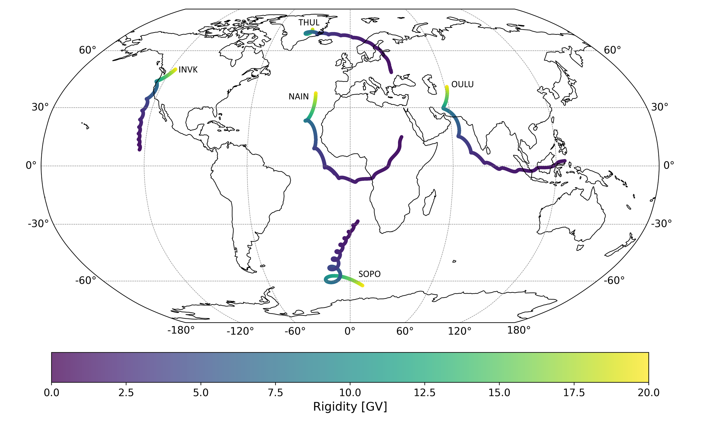
Figure 2: Asymptotic cones for the Oulu, Nain, South Pole, Thule, and Inuvik neutron monitors for the IGRF 2010 epoch and TSY89 model, with kp = 0. Latitudes and longitudes are in the geocentric coordinate system.

Trajectory

Computes and outputs the trajectory of a charged particle with a specified rigidity from a given start location on Earth. Positional information can be in any of the available coordinate systems.

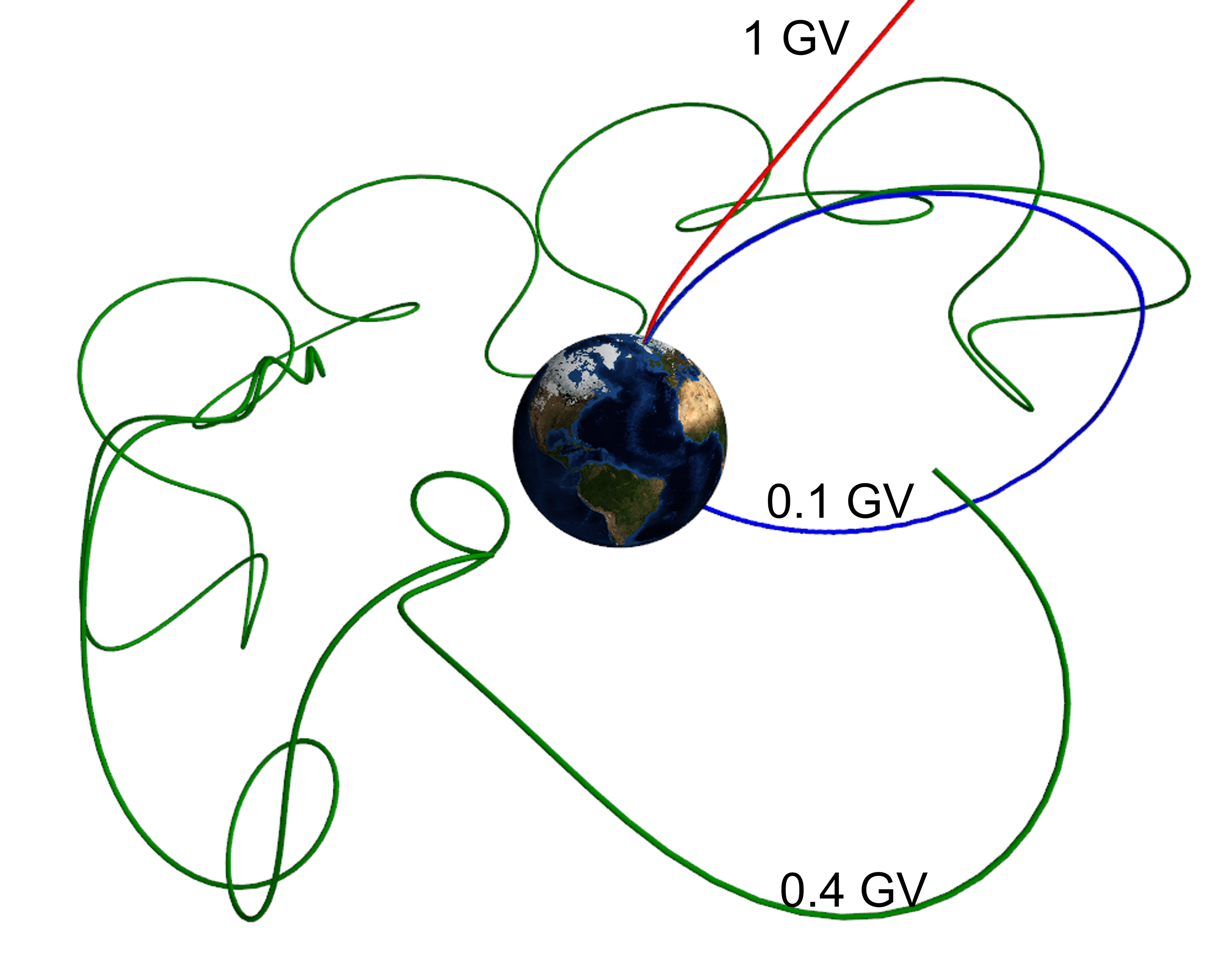
Figure 3: Computed trajectories of three cosmic rays of various rigidity values being backtraced from the Oulu neutron monitor for the IGRF 2000 and TSY89 model, with kp = 0. The 1GV particle is allowed (able to escape the magnetosphere); the 0.4GV particle is forbidden (it is trapped in the magnetosphere); and the 0.1GV is also forbidden (it returns to Earth).

Planet

Performs the cutoff function over a user-defined location grid, allowing for cutoffs for the entire globe to be computed instead of individual locations. There is the option to return the asymptotic viewing directions at each computed location by utilising a user-inputted list of rigidity levels.

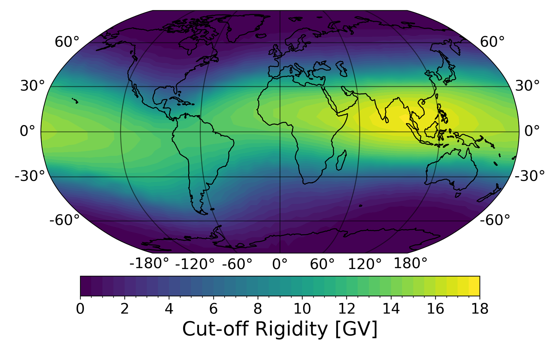Figure 4: Computed vertical effective cut-off rigidities across a 5°x5° grid of the Earth. These computations were done using the IGRF 2000 epoch and TSY89 model, with kp = 0.

Flight

Computes the cut-off rigidities along a user-defined path. The function is named Flight as it is primarily been developed for use in aviation tools, but any path can be entered. For example, the function can be applied to geomagnetic latitude surveys using positional data from a ship voyage, or it can be used to compute anisotropy and cut-off values for low-Earth orbit spacecraft. This function allows for changing altitude, location, and date values.

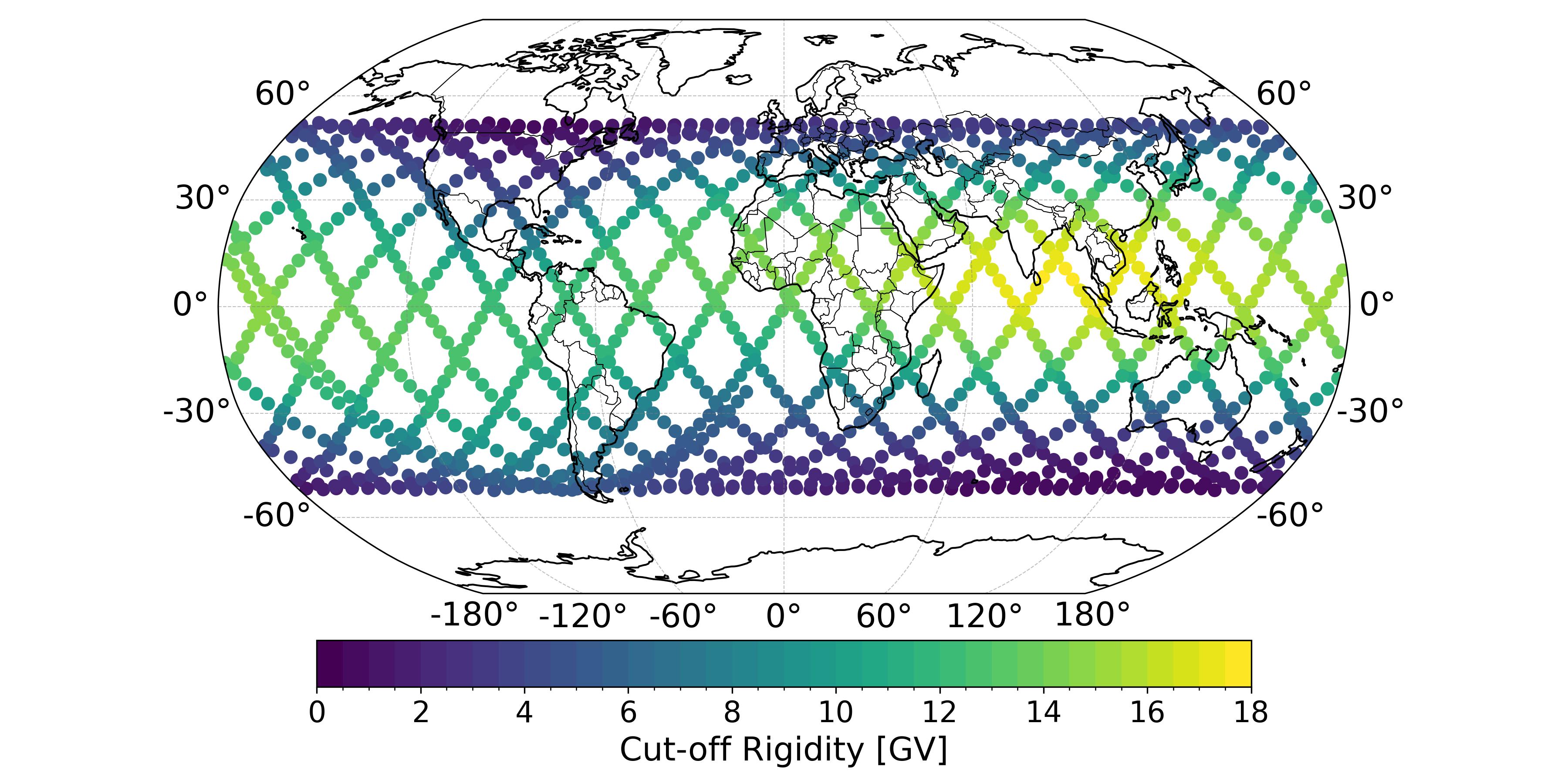
Figure 3: Computed effective vertical cut-off rigidities for the ISS between the 15th and 16th of March 2021. Geomagnetic parameters were extracted directly from OMNI for this period.

Trace

Traces the magnetic field lines around the globe or for a given location based on the geomagnetic configuration detailed by the user. It is useful for modelling the magnetosphere structure under disturbed conditions and for finding open magnetic field lines.

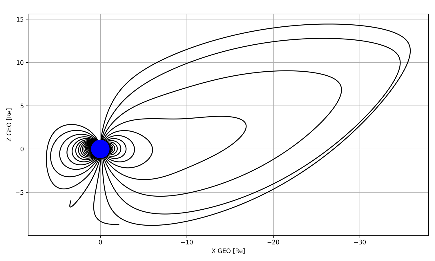Figure 5: Computation of magnetic field line configuration in the X-Z plane on January 1st 2000 12:00:00. IGRF and TSY01 models used, and input variables were obtained using the server data option within OTSO.

Coordtrans

Converts input positional information from one coordinate system to another, utilising the IRBEM library of coordinate transforms.

Magfield

Computes the total magnetic field strength at a given location depending on the user's input geomagnetic conditions. Outputs will be in the geocentric solar magnetospheric (GSM) coordinate system.

Examples

Cutoff

import OTSO

if __name__ == '__main__':
    stations_list = ["OULU", "ROME", "ATHN", "CALG"]  # list of neutron monitor stations (using their abbreviations)

    cutoff = OTSO.cutoff(
        Stations=stations_list,
        computation_params={"corenum": 1},
        datetime_params={"year": 2000, "month": 1, "day": 1, "hour": 0}
    )

    print(cutoff[0])  # dataframe output containing Ru, Rc, Rl for all input locations
    print(cutoff[1])  # text output of input variable information

Output

Ru = upper cut-off rigidity [GV]

Rc = effective cut-off rigidity [GV]

Rl = lower cut-off rigidity [GV]

    ATHN  CALG  OULU  ROME
Ru  8.98  1.14  0.72  6.35
Rc  8.33  1.07  0.71  6.07
Rl  6.31  1.02  0.59  5.37

Cone

import OTSO

if __name__ == '__main__':

    stations_list = ["OULU", "ROME", "ATHN", "CALG"]  # list of neutron monitor stations (using their abbreviations)

    cone = OTSO.cone(
        Stations=stations_list,
        computation_params={"corenum": 1},
        datetime_params={"year": 2000, "month": 1, "day": 1, "hour": 0}
    )

    print(cone[0])  # dataframe output containing asymptotic cones for all input locations
    print(cone[1])  # dataframe output containing Ru, Rc, Rl for all inputted locations
    print(cone[2])  # text output of input variable information

Output

Showing only the cone[0] output containing the asymptotic viewing directions of the input stations. Result layout is: filter;latitude;longitude. If the filter value is 1, then the particle of that rigidity has an allowed trajectory. If the filter value is NOT 1, then the particle of that rigidity has a forbidden trajectory.

      R [GV]                ATHN               CALG               OULU               ROME
0     20.000     1;-1.635;89.172   1;21.147;271.975    1;40.902;62.437     1;4.052;71.083
1     19.990     1;-1.661;89.200   1;21.131;271.973    1;40.890;62.435     1;4.027;71.101
2     19.980     1;-1.687;89.228   1;21.117;271.972    1;40.877;62.434     1;4.001;71.120
3     19.970     1;-1.713;89.256   1;21.101;271.970    1;40.865;62.432     1;3.975;71.138
4     19.960     1;-1.739;89.283   1;21.086;271.969    1;40.853;62.431     1;3.950;71.156
...      ...                 ...                ...                ...                ...
1995   0.050    -1;5.784;175.702   -1;38.217;16.098  -1;43.597;238.366   -1;3.370;219.840
1996   0.040   -1;20.165;207.726   -1;20.122;39.597  -1;24.492;229.951  -1;24.971;178.788
1997   0.030  -1;-32.777;224.618   -1;29.968;12.264  -1;17.566;214.996  -1;17.415;216.472
1998   0.020    -1;7.967;228.903   -1;33.543;96.634  -1;36.906;180.237  -1;30.685;186.313
1999   0.010   -1;19.485;224.643  -1;-4.295;338.997  -1;57.813;160.815  -1;26.726;219.327

Trajectory

import OTSO

if __name__ == '__main__':

    stations_list = ["OULU", "ROME", "ATHN", "CALG"]  # list of neutron monitor stations (using their abbreviations)

    trajectory = OTSO.trajectory(
        Stations=stations_list,
        rigidity_params={"startrigidity": 5},
        computation_params={"corenum": 1}
    )

    print(trajectory[0])  # dictionary output containing positional information for all trajectories generated starting
                         # from input stations
    print(trajectory[1])  # text output of input variable information

Output

Showing the dataframe produced for the particle originating from Oulu. Other trajectories are within the trajectory[0] dictionary. Additionally the Filter value, letting you know if the trajectory is allowed or not, and the asymptotic latitude and longitude at the end point is included.

{'NMname': 'OULU', 'trajectory':