ReachabilityAnalysis.jl
Computing reachable states of dynamical systems in Julia
Install / Use
/learn @JuliaReach/ReachabilityAnalysis.jlREADME
ReachabilityAnalysis.jl
| Documentation | Status | Community | License |
|:-----------------:|:----------:|:-------------:|:-----------:|
| ![]() |
| ![]()


![]()
 |
| ![]()
 |
|  |
|
✨ What is Reachability Analysis?
Reachability analysis is concerned with computing rigorous approximations of the set of states reachable by a dynamical system. In the scope of this package are systems modeled by continuous or hybrid dynamical systems, where the dynamics changes with discrete events. Systems are modelled by ordinary differential equations (ODEs) or semi-discrete partial differential equations (PDEs), with uncertain initial states, uncertain parameters or non-deterministic inputs.
The library is oriented towards a class of numerical methods known as set propagation techniques: to compute the set of states reachable by continuous or hybrid systems, such methods iteratively propagate a sequence of sets starting from the set of initial states, according to the systems' dynamics.
See our Frequently asked questions (FAQ) section for pointers to the relevant literature, related tools and more.
🎯 Table of Contents
🎨 Features
:checkered_flag: Quickstart
:blue_book: Publications
📜 Citation
💾 Installation
Open a Julia session and activate the
pkg mode (to activate the pkg mode in Julia's REPL, type ],
and to leave it, type <backspace>), and enter:
pkg> add ReachabilityAnalysis
📙 Documentation
See the Reference Manual for introductory material, examples and API references.
📌 Need help? Have any question, or wish to suggest or ask for a missing feature?
Do not hesitate to open an issue or join the JuliaReach Zulip chat: ![]() . You can also send an email to the developers.
. You can also send an email to the developers.
🎨 Features
The following types of systems are supported (click on the left arrow to display a list of examples):
<details> <summary> Continuous ODEs with linear dynamics :heavy_check_mark: </summary> <p> <a href="https://juliareach.github.io/ReachabilityAnalysis.jl/dev/generated_examples/OpAmp/">Operational amplifier</a> </p> <p> <a href="https://juliareach.github.io/ReachabilityModels.jl/dev/models/heat/">Heat</a> </p> <p> <a href="https://juliareach.github.io/ReachabilityAnalysis.jl/dev/generated_examples/ISS/">ISS</a> </p> <p> <a href="https://juliareach.github.io/ReachabilityModels.jl/dev/models/motor">Motor</a> </p> <p> <a href="https://juliareach.github.io/ReachabilityAnalysis.jl/dev/generated_examples/Building/">Building</a> </p> </details> <details> <summary> Continuous ODEs with non-linear dynamics :heavy_check_mark: </summary> <p> <a href="https://juliareach.github.io/ReachabilityAnalysis.jl/dev/generated_examples/Quadrotor/">Quadrotor</a> </p> <p> <a href="https://juliareach.github.io/ReachabilityAnalysis.jl/dev/generated_examples/Brusselator/">Brusselator</a> </p> <p> <a href="https://juliareach.github.io/ReachabilityAnalysis.jl/dev/generated_examples/SEIR/">SEIR model</a> </p> <p> <a href="https://juliareach.github.io/ReachabilityModels.jl/dev/models/robot_arm">Robot arm</a> </p> </details> <details> <summary> Continuous ODEs with parametric uncertainty :heavy_check_mark: </summary> <p> <a href="https://juliareach.github.io/ReachabilityAnalysis.jl/dev/generated_examples/TransmissionLine/">Transmission line</a> </p> <p> <a href="https://juliareach.github.io/ReachabilityAnalysis.jl/dev/generated_examples/LotkaVolterra/">Lotka-Volterra</a> </p> </details> <details> <summary> Hybrid systems with piecewise-affine dynamics :heavy_check_mark: </summary> <p> <a href="https://juliareach.github.io/ReachabilityAnalysis.jl/dev/generated_examples/Platoon/">Platooning</a> </p> <p> <a href="https://juliareach.github.io/ReachabilityModels.jl/dev/models/bouncing_ball">Bouncing ball</a> </p> <p> <a href="https://juliareach.github.io/ReachabilityModels.jl/dev/models/navigation_system">Navigation system</a> </p> <p> <a href="https://juliareach.github.io/ReachabilityModels.jl/dev/models/thermostat">Thermostat</a> </p> </details> <details> <summary> Hybrid systems with non-linear dynamics :heavy_check_mark: </summary> <p> <a href="https://juliareach.github.io/ReachabilityAnalysis.jl/dev/generated_examples/Spacecraft/">Spacecraft</a> </p> <p> <a href="https://juliareach.github.io/ReachabilityModels.jl/dev/models/cardiac_cell">Cardiatic cell</a> </p> <p> <a href="https://juliareach.github.io/ReachabilityModels.jl/dev/models/powertrain_control">Powetrain control</a> </p> <p> <a href="https://juliareach.github.io/ReachabilityModels.jl/dev/models/spiking_neuron">Spiking neuron</a> </p> <p> <a href="https://juliareach.github.io/ReachabilityModels.jl/dev/models/bouncing_ball_nonlinear">Bouncing ball</a> </p> </details> <details> <summary> Hybrid systems with clocked linear dynamics :heavy_check_mark: </summary> <p> <a href="https://github.com/JuliaReach/ARCH2020_AFF_RE/blob/master/models/EMBrake/embrake.jl">Electromechanic break</a> </p> <p> <a href="https://juliareach.github.io/ReachabilityModels.jl/dev/models/clocked_thermostat">Clocked thermostat</a> </p> </details>:checkered_flag: Quickstart
In less than 15 lines of code, we can formulate, solve and visualize the set of states reachable by the Duffing oscillator starting from any initial condition
with position in the interval 0.9 .. 1.1 and velocity in -0.1 .. 0.1.
using ReachabilityAnalysis, Plots

const ω = 1.2
const T = 2 * pi / ω

@taylorize function duffing!(du, u, p, t)
    local α = -1.0
    local β = 1.0
    local δ = 0.3
    local γ = 0.37

    x, v = u
    f = γ * cos(ω * t)

    # write the nonlinear differential equations defining the model
    du[1] = u[2]
    du[2] = -α*x - δ*v - β*x^3 + f
end

# set of initial states
X0 = Hyperrectangle(low=[0.9, -0.1], high=[1.1, 0.1])

# formulate the initial-value problem
prob = @ivp(x' = duffing!(x), x(0) ∈ X0, dim=2)

# solve using a Taylor model set representation
sol = solve(prob, tspan=(0.0, 20*T), alg=TMJets21a());

# plot the flowpipe in state-space
plot(sol, vars=(1, 2), xlab="x", ylab="v", lw=0.5, color=:red)
🐾 Examples
| | |
|:--------:|:-----:|
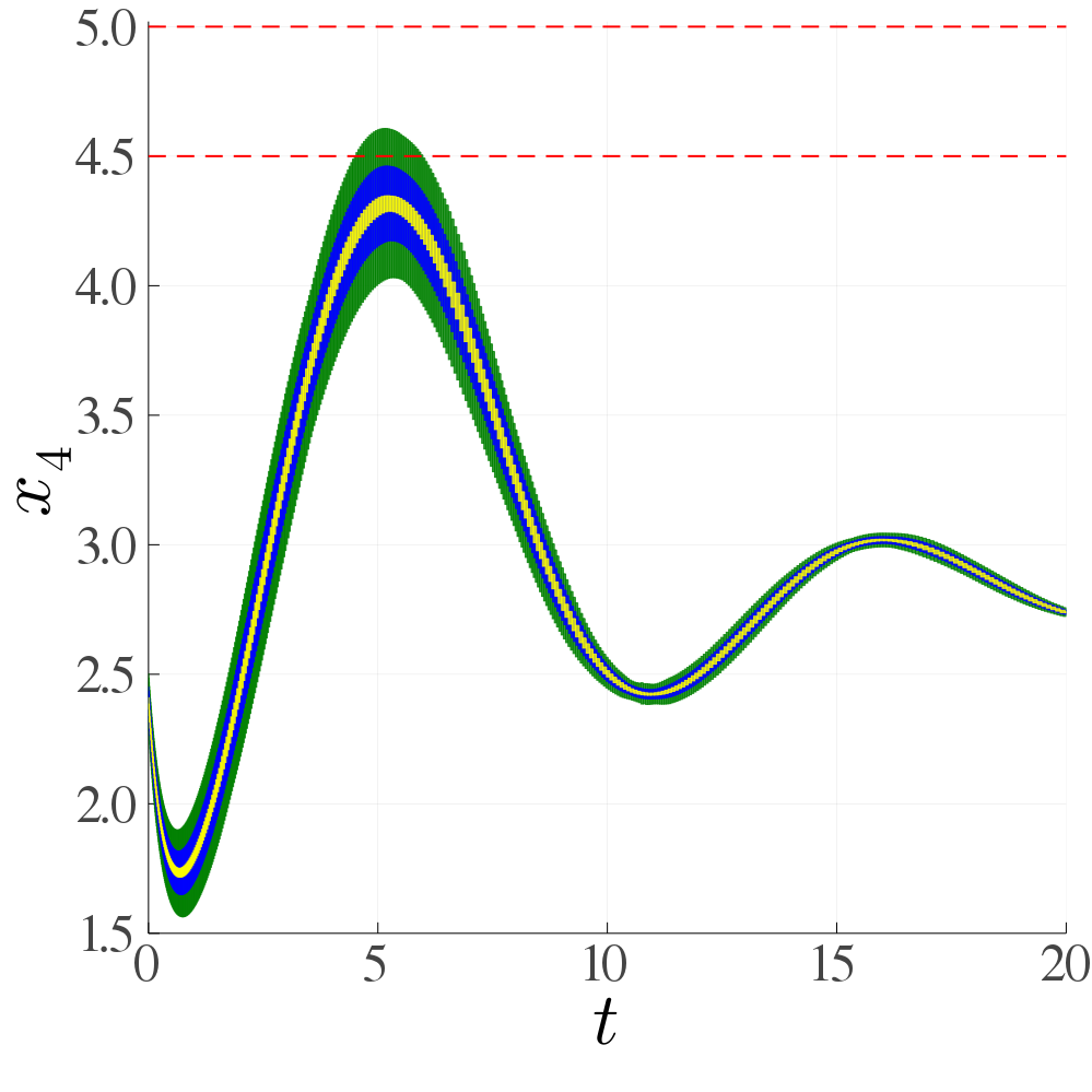
| 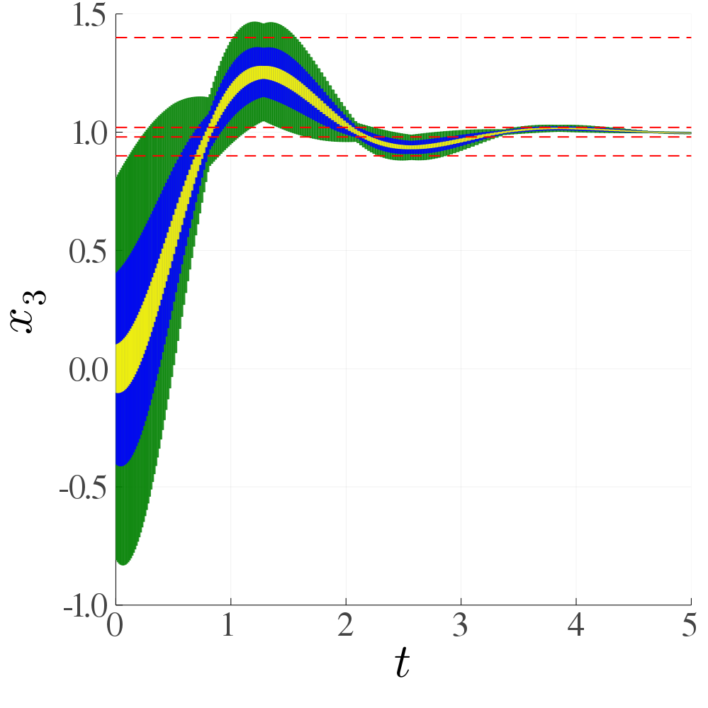 Quadrotor altitude control |
 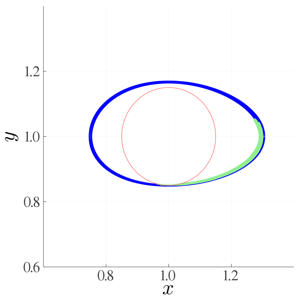 Lotka-Volterra with tangential guard crossing|
| | |
|
Lotka-Volterra with tangential guard crossing|
| | |
|  [Laub-Loomis model](https://juliareach.github.io/ReachabilityAnalysis.j
