PyALE <img src="https://raw.githubusercontent.com/DanaJomar/PyALE/master/.github/pyale-hex-thicker.png" align="right" height="256" alt="pyale logo"/>

ALE: Accumulated Local Effects <br> A python implementation of the ALE plots based on the implementation of the R package ALEPlot

Installation:

Via pip pip install PyALE

Features:

The end goal is to be able to create the ALE plots whether was the feature numeric or categorical.

For numeric features:

The package offers the possibility to

Compute and plot the effect of one numeric feature (1D ALE)
- including the option to compute a confidence interval of the effect.
Compute and plot the effect of two numeric features (2D ALE)

For categorical features:

Since python models work with numeric features only, categorical variables are often encoded by one of two methods, either with integer encoding (when the categories have a natural ordering of some sort e.g., days of the week) or with one-hot-encoding (when the categories do not have ordering e.g., colors). The package offers the option to compute and plot the effect of such features, including the option to compute a confidence interval of the effect. In this case the use has two options:

For integer encoding: the user can plot the effect of the feature as a discrete feature
- does not need additional preparation steps
For one-hot-encoding: or any other custom encoding, the package, starting from version 1.1, offers the possibility to pass a custom encoding function to categorical (or string) features.
- in this case the user must provide
  - a function that encodes the raw feature
  - a data set that includes the raw feature instead of the encoded one (including all other features used for training)
  - a list of all predictors used for training the model

The package by default uses the ordering assigned to the given categorical feature, however, if the feature does not have an assigned ordering, then the categories of the feature will be ordered by their similarities based on the distribution of the other features in each category.

Usage with examples:

First prepare the data and train a model.
- To explore the different features in this package, we choose one categorical feature to one-hot-encode, and we'll use integer encoding for the rest.
- Full code and other examples can be found in Examples
For the following examples we train a random forest to predict the price of diamonds with the following data
```
X[features]
```
| carat | cut_code | clarity_code | depth | table | x | y | z | D | E | F | G | H | I | J | | ----- | -------- | ------------ | ----- | ----- | ---- | ---- | ---- | ---- | ---- | ---- | ---- | ---- | ---- | ---- | | 0.23 | 4 | 1 | 61.5 | 55.0 | 3.95 | 3.98 | 2.43 | 0.0 | 1.0 | 0.0 | 0.0 | 0.0 | 0.0 | 0.0 | | 0.21 | 3 | 2 | 59.8 | 61.0 | 3.89 | 3.84 | 2.31 | 0.0 | 1.0 | 0.0 | 0.0 | 0.0 | 0.0 | 0.0 | | 0.23 | 1 | 4 | 56.9 | 65.0 | 4.05 | 4.07 | 2.31 | 0.0 | 1.0 | 0.0 | 0.0 | 0.0 | 0.0 | 0.0 | | 0.29 | 3 | 3 | 62.4 | 58.0 | 4.20 | 4.23 | 2.63 | 0.0 | 0.0 | 0.0 | 0.0 | 0.0 | 1.0 | 0.0 | | 0.31 | 1 | 1 | 63.3 | 58.0 | 4.34 | 4.35 | 2.75 | 0.0 | 0.0 | 0.0 | 0.0 | 0.0 | 0.0 | 1.0 |
import the generic function ale from the package
```
from PyALE import ale
```
start analysing the effects of your features
- 1D ALE plot for numeric continuous feature
```
## 1D - continuous - no CI
ale_eff = ale(
    X=X[features], model=model, feature=["carat"], grid_size=50, include_CI=False
)
```
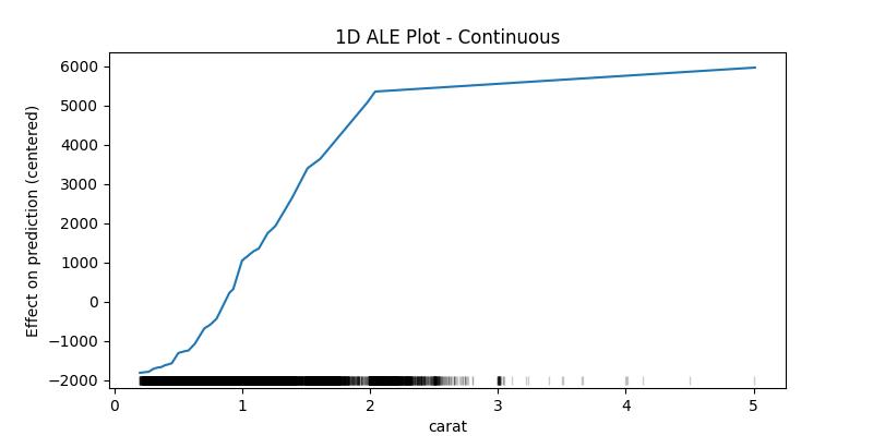
  The confidence intervals around the estimated effects are specially important when the sample data is small, which is why as an example plot for the confidence intervals we'll take a random sample of the dataset
```
## 1D - continuous - with 95% CI
random.seed(123)
X_sample = X[features].loc[random.sample(X.index.to_list(), 1000), :]
ale_eff = ale(
    X=X_sample, model=model, feature=["carat"], grid_size=50, include_CI=True, C=0.95
)
```
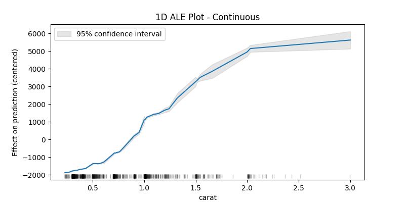
- 1D ALE plot for numeric discrete feature
```
## 1D - discrete
ale_eff = ale(X=X[features], model=model, feature=["cut_code"])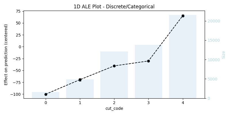
```
- 1D ALE plot for [one-hot-encoded] categorical feature
  
  In this case, it is not enough to use X[features] (that was used for training), because it does not contain the original feature, we have to replace the encoding with the raw feature, and then we need to pass a custom encoding function (in our example the functiononehot_encode) and a list or array of all used predictors (in our example the list features)
```
## remove the one-hot-encoding columns and add the original -raw- feature
## since X already has the raw feature it is enough to drop its encoding columns 
X_feat_raw = X.drop(coded_feature.columns.to_list(), axis=1, inplace=False).copy()

## 1D - categorical
ale_eff = ale(
    X=X_feat_raw,
    model=model,
    feature=["color"],
    encode_fun=onehot_encode,
    predictors=features,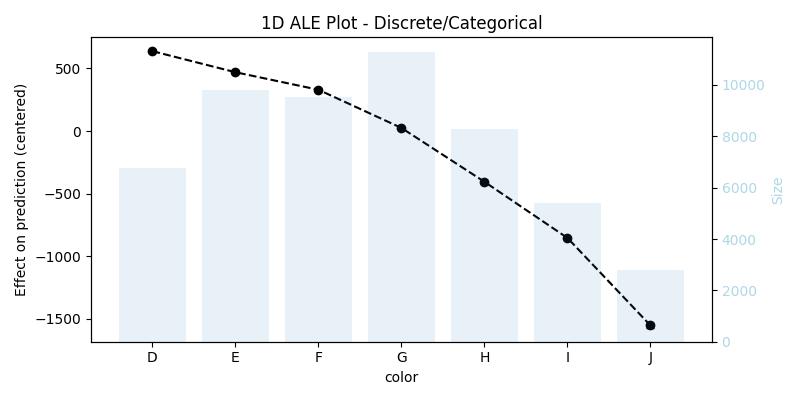
)
```
Note that the function ale has detected the right feature type in all three cases, however, the user can always specify the feature type if she/he thinks that the function did not detect the expected type.

2D ALE plot for numeric features

## 2D - continuous
ale_eff = ale(X=X[features], model=model, feature=["z", "table"], grid_size=100)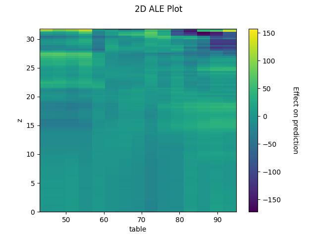

2D ALE Plot

Interpretation:

random.seed(123)
X_sample = X[features].loc[random.sample(X.index.to_list(), 1000), :]
ale_contin = ale(
    X=X_sample,
    model=model,
    feature=["carat"],
    feature_type="continuous",
    grid_size=5,
    include_CI=True,
    C=0.95,
)

1D ALE Plot

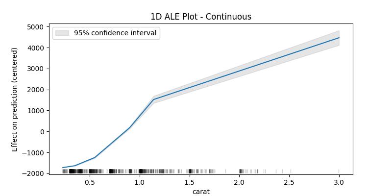
For continuous variables the algorithm cuts the feature to bins starting from the minimum value and ending with the maximum value of the feature, then computes the average difference in prediction when the value of the feature moves between the edges of each bin, finally returns the centered cumulative sum of these averages (and the confidence interval of the differences - optional).

ale_contin

| carat | eff | size | lowerCI_95% | upperCI_95% | | ------ | ----------- | ------ | ----------- | ----------- | | 0.23 |-1721.408141 | 0.0 | NaN | NaN | | 0.35 |-1633.405685 | 203.0 | -1650.042600 | -1616.768770 | | 0.55 |-1242.989786 | 204.0 | -1275.489577 | -1210.489995 | | 0.90 | 176.838662 | 213.0 | 125.162929 | 228.514394 | | 1.14 | 1521.617690 | 182.0 | 1351.287932 | 1691.947448 | | 3.00 | 4467.185422 | 198.0 | 4115.599415 | 4818.771429 |

What interests us when interpreting the results is the difference in the effect between the edges of the bins, in this example one can say that the value of the prediction increases by approximately 2946 (4467 - 1521) when the carat increases from 1.14 to 3.00, as can be seen in the last two lines. With this in mind we can see that the values of the confidence interval only makes sense starting from the second value (the upper edge of the first bin) and could also be compared with the eff value of the previous row as to give an idea of how much this difference can fluctuate (e.g., for the bin (1.14, 3.00] between 2764 and 3127 with 95% certainty).

The lower edge of the first bin is in fact the minimum value of the feature in the given data, and it belongs to the first bin (unlike the following bins which contain the upper edge but not the lower). The size column contains the number of data points in the bin ending with the feature value in the corresponding row and starting with value before it (e.g., the bin (1.14, 3.00] has 198 data points). The rug at the bottom of the generated plot shows the distribution of the data points.

For categoricals or variables with discrete values the interpretation is similar and we also get the average difference in prediction, but instead of bins each value will be replaced once with the value before it and once with the value after it.

ale_discr = ale(
    X=X_sample,
    model=model,
    feature=["cut_code"],
    feature_type="discrete",
    include_CI=True,
    C=0.95,
)

![1D ALE Plot](https://raw.githubusercontent.com/DanaJomar/PyALE/master/examples/plots/interpret

PyALE

Install / Use

README