Log Periodic Power Law Singularity (LPPLS) Model

lppls is a Python module for fitting the LPPLS model to data.

Overview

The LPPLS model provides a flexible framework to detect bubbles and predict regime changes of a financial asset. A bubble is defined as a faster-than-exponential increase in asset price, that reflects positive feedback loop of higher return anticipations competing with negative feedback spirals of crash expectations. It models a bubble price as a power law with a finite-time singularity decorated by oscillations with a frequency increasing with time.

Try the demo:

Here is the model:

E[ln\ p(t)] = A + B(t_c-t)^{m}+C(t_c-t)^{m}\cos(\omega\ ln(t_c-t) - \phi)

where:

• $E[ln\ p(t)]$: expected log price at the date of the termination of the bubble
• $t_c$: critical time (date of termination of the bubble and transition in a new regime)
• $A$: expected log price at the peak when the end of the bubble is reached at $t_c$
• $B$: amplitude of the power law acceleration
• $C$: amplitude of the log-periodic oscillations
• $m$: degree of the super exponential growth
• $\omega$: scaling ratio of the temporal hierarchy of oscillations
• $\phi$: time scale of the oscillations

The model has three components representing a bubble. The first, $A+B(t_c-t)^{m}$, handles the hyperbolic power law. For $m$ < 1 when the price growth becomes unsustainable, and at $t_c$ the growth rate becomes infinite. The second term, $C(t_c-t)^{m}$, controls the amplitude of the oscillations. It drops to zero at the critical time $t_c$. The third term, $\cos(\omega\ ln(t_c-t) - \phi)$, models the frequency of the oscillations. They become infinite at $t_c$.

Important links

• Official source code repo: https://github.com/Boulder-Investment-Technologies/lppls
• Download releases: https://pypi.org/project/lppls/
• Issue tracker: https://github.com/Boulder-Investment-Technologies/lppls/issues

Installation

Dependencies

lppls requires:

• Python (>= 3.10)
• CMA-ES (>= 3.3.0)
• Matplotlib (>= 3.5.0)
• Numba (>= 0.56.0)
• NumPy (>= 1.23.0)
• Pandas (>= 1.5.0)
• SciPy (>= 1.9.0)
• Scikit-learn (>= 1.2.0)
• tqdm (>= 4.64.0)
• Xarray (>= 2024.1.0)

User installation

pip install -U lppls

Example Use

from lppls import lppls, data_loader
import numpy as np
import pandas as pd
from datetime import datetime as dt
%matplotlib inline

# read example dataset into df 
data = data_loader.nasdaq_dotcom()

# convert time to ordinal
time = [pd.Timestamp.toordinal(dt.strptime(t1, '%Y-%m-%d')) for t1 in data['Date']]

# create list of observation data
price = np.log(data['Adj Close'].values)

# create observations array (expected format for LPPLS observations)
observations = np.array([time, price])

# set the max number for searches to perform before giving-up
# the literature suggests 25
MAX_SEARCHES = 25

# instantiate a new LPPLS model with the Nasdaq Dot-com bubble dataset
lppls_model = lppls.LPPLS(observations=observations)

# fit the model to the data and get back the params
tc, m, w, a, b, c, c1, c2, O, D = lppls_model.fit(MAX_SEARCHES)

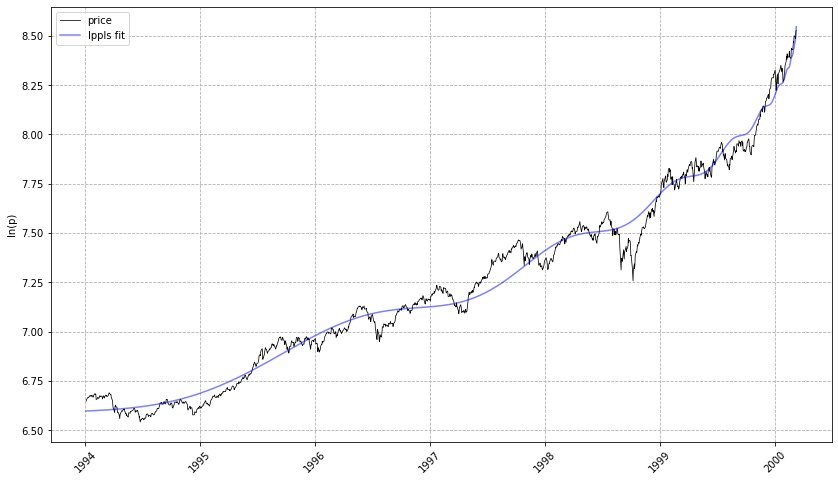
# visualize the fit
lppls_model.plot_fit()

# should give a plot like the following...

# compute the confidence indicator
res = lppls_model.mp_compute_nested_fits(
    workers=8,
    window_size=120, 
    smallest_window_size=30, 
    outer_increment=1, 
    inner_increment=5, 
    max_searches=25,
    # filter_conditions_config={} # not implemented in 0.6.x
)

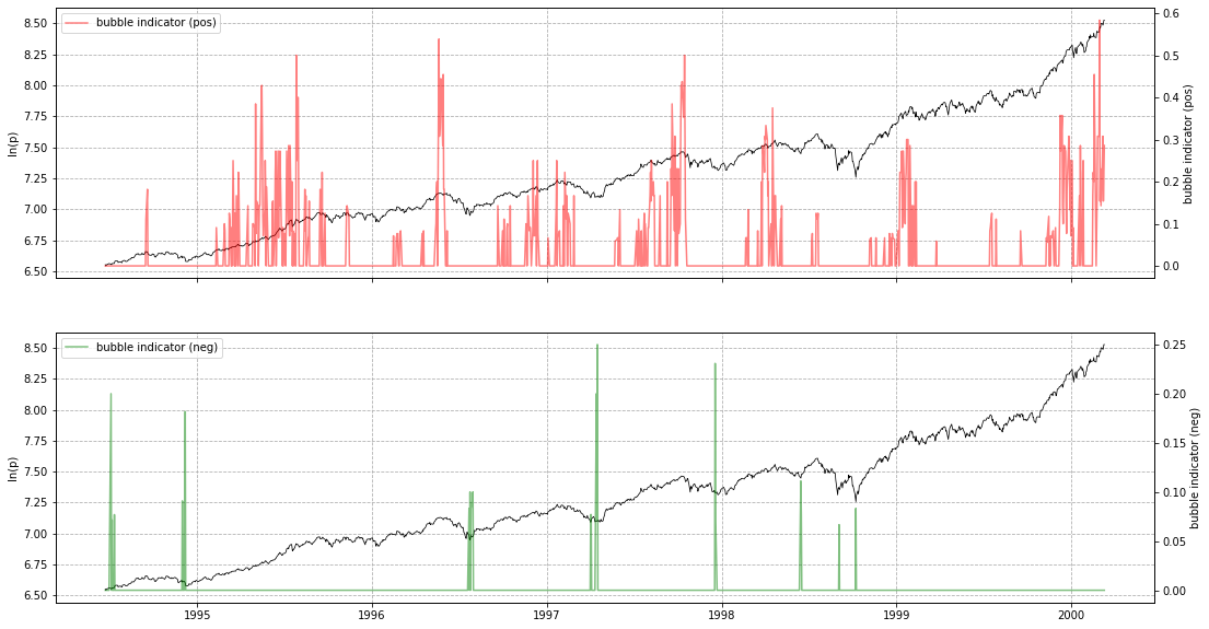
lppls_model.plot_confidence_indicators(res)
# should give a plot like the following...

If you wish to store res as a pd.DataFrame, use compute_indicators.

<details> <summary>Example</summary>

res_df = lppls_model.compute_indicators(res)
res_df
# gives the following...

<img src="https://raw.githubusercontent.com/Boulder-Investment-Technologies/lppls/master/img/compute_indicator_df.png" width="500"/> </details>

Quantile Regression

Based on the work in Zhang, Zhang & Sornette 2016, quantile regression for LPPLS uses the L1 norm (sum of absolute differences) instead of the L2 norm and applies the q-dependent loss function during calibration. Please refer to the example usage here.

Lagrange Regularization for Bubble Start Time Detection

The lppls library includes a method for determining the start time of a financial bubble using Lagrange regularization. This technique, inspired by the work of Demos & Sornette (2017), addresses the challenge of model overfitting when the bubble's inception is unknown.

By introducing a regularization term to the normalized sum of squared residuals, the method objectively identifies the optimal fitting window size. This allows for a more robust and data-driven estimation of the bubble's start time without requiring exogenous information, which is a significant improvement over previous approaches.

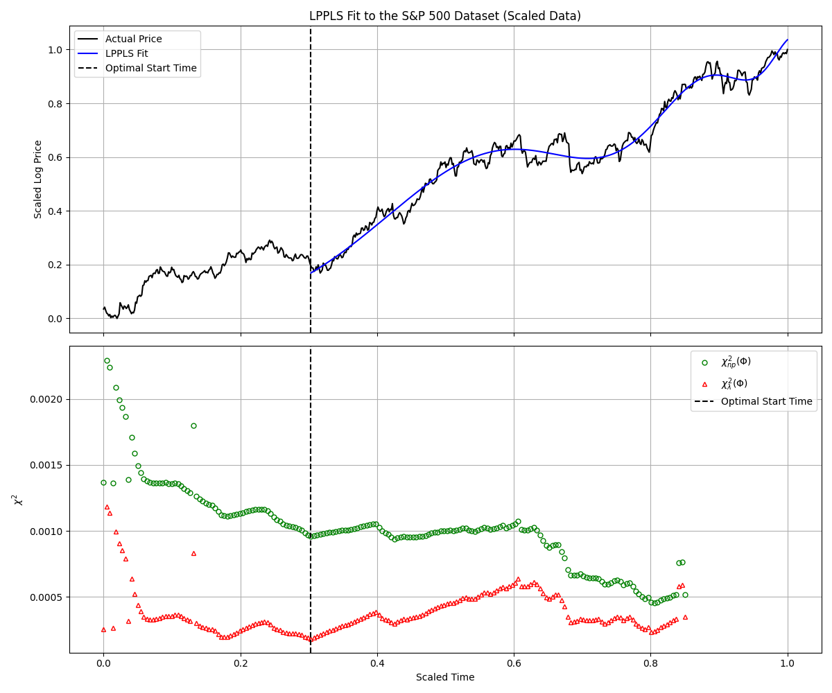
This functionality is available through the detect_bubble_start_time_via_lagrange method. For detailed usage, please refer to the tutorial here.

Other Search Algorithms

Shu and Zhu (2019) proposed CMA-ES for identifying the best estimation of the three non-linear parameters ($t_c$, $m$, $\omega$).

The CMA-ES rates among the most successful evolutionary algorithms for real-valued single-objective optimization and is typically applied to difficult nonlinear non-convex black-box optimization problems in continuous domain and search space dimensions between three and a hundred. Parallel computing is adopted to expedite the fitting process drastically.

This approach has been implemented in a subclass and can be used as follows... Thanks to @paulogonc for the code.

from lppls import lppls_cmaes
lppls_model = lppls_cmaes.LPPLSCMAES(observations=observations)
tc, m, w, a, b, c, c1, c2, O, D = lppls_model.fit(max_iteration=2500, pop_size=4)

Performance Note: this works well for single fits but can take a long time for computing the confidence indicators. More work needs to be done to speed it up.

References

• Filimonov, V. and Sornette, D. A Stable and Robust Calibration Scheme of the Log-Periodic Power Law Model. Physica A: Statistical Mechanics and its Applications. 2013
• Shu, M. and Zhu, W. Real-time Prediction of Bitcoin Bubble Crashes. 2019.
• Sornette, D. Why Stock Markets Crash: Critical Events in Complex Financial Systems. Princeton University Press. 2002.
• Sornette, D. and Demos, G. and Zhang, Q. and Cauwels, P. and Filimonov, V. and Zhang, Q., Real-Time Prediction and Post-Mortem Analysis of the Shanghai 2015 Stock Market Bubble and Crash (August 6, 2015). Swiss Finance Institute Research Paper No. 15-31.
• Demos, G. and Sornette, D. Lagrange regularisation approach to compare nested data sets and determine objectively financial bubbles' inceptions. 2017. arXiv:1707.07162
• Zhang, Q., Zhang, Q., and Sornette, D. Early Warning Signals of Financial Crises with Multi-Scale Quantile Regressions of Log-Periodic Power Law Singularities. PLOS ONE. 2016. DOI:10.1371/journal.pone.0165819